Scattering on a two-level system

In the following, we show that with our framework, we can reproduce the theoretical results obtained in Le Jeannic, et al. Nat. Phys. 18, 1191–1195 (2022)

In many of the examples considered so far, we only consider a single waveguide that serves as both input and output, thus only allowing for only one-sided cavities or quantum systems at the end of a waveguide. A more realistic scenario is having a waveguide with a quantum system in the middle. Here an incoming waveguide carrying an excitation could scatter on the quantum system, and one would have excitations going away from the quantum system in both the first and latter part of the waveguide, as illustrated here:^[1]

`alt text`

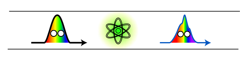
A way to model this scenario is to have two waveguides: a waveguide to the left and the right, describing the first half of the waveguide and the latter half. For this, we use WaveguideBasis but with an extra argument specifying that we need two waveguides (see Multiple Waveguides for an introduction). We initialize WaveguideBasis with two waveguides and a basis for the atom (note that a fockbasis with only one excitation allowed is the same as a two-level-system):

times = 0:0.1:10
dt = times[2] - times[1]
bw = WaveguideBasis(2,2,times)
be = FockBasis(1)

We then define the operators for the interaction between atom and waveguide as (notice the second argument in create(bw,1) that defines which waveguide we are addressing):

wdLa = create(bw,1) ⊗ destroy(be)
adwL = destroy(bw,1) ⊗ create(be)
wdRa = create(bw,2) ⊗ destroy(be)
adwR = destroy(bw,2) ⊗ create(be)

where $\mathrm{wdLa} = w_L ^\dagger a$, $\mathrm{wdRa} = w_R ^\dagger a$, $\mathrm{adwL} = w_L a^\dagger$, and $\mathrm{adwR} = w_R a^\dagger$. In this example, we, however, also need an interaction between the waveguides. Therefore we define the creation and annihilation operators:

wdL = create(bw,1) ⊗ identityoperator(be)
wL = destroy(bw,1) ⊗ identityoperator(be)
wdR = create(bw,2) ⊗ identityoperator(be)
wR = destroy(bw,2) ⊗ identityoperator(be)

The interaction should carry over the momentum of the left waveguide into the waveguide on the right, and the interaction should therefore model a SWAP gate. This corresponds to $V = \pi /2$ and thus we have the interaction Hamiltonian:

V = pi/2
κ1 = 1
κ2 = 1
H = im*sqrt(κ1/dt)*(adwL-wdLa) + im*sqrt(κ2/dt)*(wdRa-adwR) + V/dt *(wdR*wL + wdL* wR)

We can now study how single or two-photon states scatter on the atom. We define the initial one-photon or two-photon Gaussian state and solve it using the defined Hamiltonian:

ξ₁(t1,σ,t0) = sqrt(2/σ)* (log(2)/pi)^(1/4)*exp(-2*log(2)*(t1-t0)^2/σ^2)
ξ₂(t1,t2,σ1,σ2,t0) = ξ₁(t1,σ1,t0) * ξ₁(t2,σ2,t0)
w = 1
t0 = 5
ψ1 = onephoton(bw,1,ξ₁,w,t0) ⊗ fockstate(be,0)
ψ2 = twophoton(bw,1,ξ₂,w,w,t0) ⊗ fockstate(be,0)
ψScat1 = waveguide_evolution(times,ψ1,H)
ψScat2 = waveguide_evolution(times,ψ2,H)

┌ Warning: Initial waveguidestate is not normalized. Consider passing norm=true to the state generation function.
└ @ WaveguideQED ~/work/WaveguideQED.jl/WaveguideQED.jl/src/solver.jl:84

Viewing the scattered states is then done using TwoPhotonView and the index for the corresponding waveguide. Giving two indices returns instead the combined single photon state in both waveguides $\sum_{j,k} \ket{1_j}_1 \ket{1_k}_2$:

ψ2LeftScat = TwoPhotonView(ψScat2,1,[:,1])
ψ2RightScat = TwoPhotonView(ψScat2,2,[:,1])
ψ2LeftRightScat = TwoPhotonView(ψScat2,2,1,[:,1])

For the single-photon states, we have to calculate the two-time scattered distribution as:

ψ1LeftScat = zeros(ComplexF64,(length(times),length(times)))
ψ1RightScat = zeros(ComplexF64,(length(times),length(times)))
ψ1LeftRightScat = zeros(ComplexF64,(length(times),length(times)))
ψ1Right = OnePhotonView(ψScat1,2,[:,1])
ψ1Left = OnePhotonView(ψScat1,1,[:,1])

for i in eachindex(times)
    for j in eachindex(times)
        ψ1LeftScat[i,j] = ψ1Left[i]*ψ1Left[j]
        ψ1RightScat[i,j] = ψ1Right[i]*ψ1Right[j]
        ψ1LeftRightScat[i,j] = ψ1Left[i]*ψ1Right[j]
    end
end

Finally, we can plot the scattered wavefunctions, and we note that this matches Fig. 3 in Ref.^[1]:

fig,axs = subplots(3,2,figsize=(6,9))
plot_list = [ψ2RightScat,ψ2LeftScat,ψ2LeftRightScat,ψ1RightScat,ψ1LeftScat,ψ1LeftRightScat]
for (i,ax) in enumerate(axs)
    plot_twophoton!(ax,plot_list[i],times)
end
axs[1].set_ylabel("\$C^{RR}\$ \n t2 [a.u]")
axs[2].set_ylabel("\$C^{LL}\$ \n t2 [a.u]")
axs[3].set_ylabel("\$C^{LR}\$ \n t2 [a.u]")
axs[3].set_xlabel("t1 [a.u]")
axs[6].set_xlabel("t1 [a.u]")
plt.tight_layout()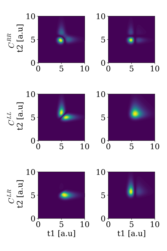

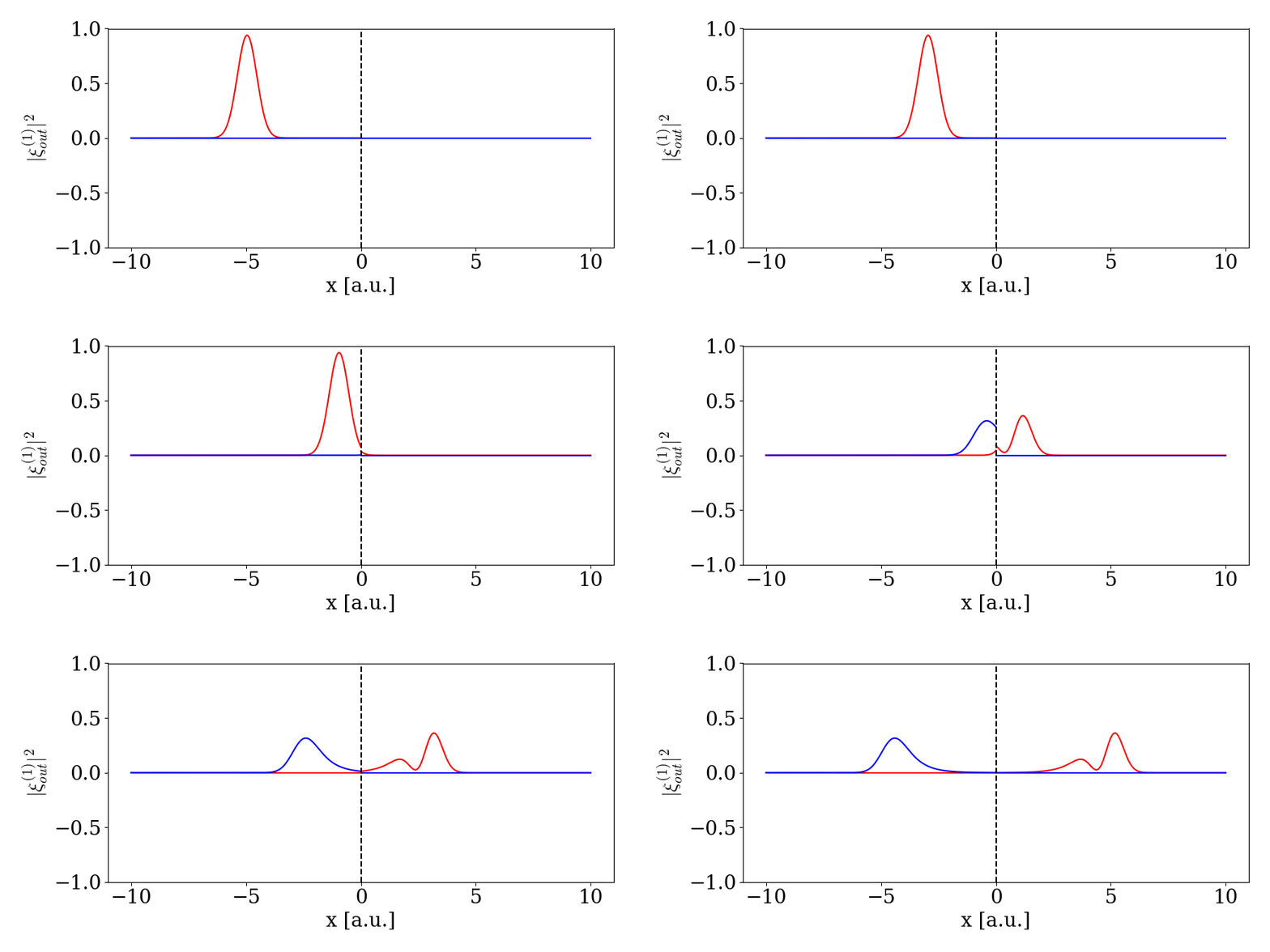
lodahl

If we consider the single photon state, we can also visualize the temporal evolution as:

alt text

1[3]