This notebook can be found on github

Simultaneous Lasing, Cooling and Trapping

In this example, we investigate simulatenous cooling and lasing of a superradiant laser. The superradiant laser operates in the bad cavity regime, i.e. the linewidth of the lasing transition $\Gamma$ is much smaller than the linewidth of the cavity $\kappa$. Usually, this is achieved by using a narrow atomic transitions, e.g. the clock transition of Strontium $(\Gamma \approx 1\mathrm{mHz})$. The advantage of a superradiant clock laser is its very narrow linewidth but also robustness against noise. In a simple model we describe the superradiant laser by $N$ incoherently pumped two-level atoms inside a cavity, and additionally we include motion along the cavity axis within a semicalssical treatment. The Hamiltonian of the system is $H = \hbar \Delta a^\dagger a + \hbar \sum_{i = 1}^{N} g(r_i) [ a \sigma_{i}^{+} + a^{\dagger} \sigma_{i}^{-}]$, where $\Delta = \omega_c - \omega_a$ is the detuing between the cavity resonance frequeny $ω_c$ and the atomic transition frequency $ω_a$. The position-dependent cavity-atom coupling of the $i$-th atoms is given by $g(r_i) = g \cos(kr_i)$, with $k$ the wavevector of the cavtiy photons. The cavity field is described by the bosonic creation and annihilation operators $a^{\dagger}$ and $a$, respectively, and the identical two-level atoms are characterized by the atomic excitation and deexcitation operators $\sigma^+$ and $\sigma^-$, respectively. The atomic decay, the photon losses through the cavity mirrors, and the incoherent pump are modeled by their corresponding Liouvillian operators, $\mathcal{L}_{\text{sp}}[\rho] = \frac{1}{2} \Gamma \sum_{i}(2 \sigma_i^- \rho \sigma_i^+ - \sigma_i^+ \sigma_i^- \rho - \rho \sigma_i^+ \sigma_i^-)$,

$\mathcal{L}_{\text{cav}}[\rho] = \frac{1}{2} \kappa (2 a \rho a^\dagger - a^\dagger a \rho - \rho a^\dagger a)$

and

$\mathcal{L}_{\text{pump}}[\rho] = \frac{1}{2} R \sum_{i} (2 \sigma^+_i \rho \sigma^-_i - \sigma^-_i \sigma^+_i \rho - \rho \sigma^-_i \sigma^+_i )$, with the incoherent pump rate $R$. To obtain the equations for the particles' semiclassical motion we use the Ehrenfest theorem leading to $\dot{r}_i = 2 \omega_{\text{r}} p_i$

and

$\dot{p}_i = 2 g \sin(k r_i) \langle a \sigma_{i}^{+} + a^{\dagger} \sigma_{i}^{-} \rangle$, where $p_i$ is the momentum of the $i$-th particle and $\omega_r = \hbar k^2/2m$ the recoil frequency. The time evolution of the system described above can be calculated by using the implemented semiclassical master equation. First we import the needed libraries and define the variables, Hilbertspaces and operators of the system.

using QuantumOpticsusing PyPlotusing OrdinaryDiffEqusing Interpolations

n_p = 3 #photonen cutoffN_a = 2 #number of atoms#all variables and parameters are given in units of the following threeΓ = 1.0 #spontaneous emission ratek = 1.0 #wavevector of the atom transition and the cavity fieldħ = 1.0 #Planck constantω_r = 0.1Γ #recoil frequencyΔ = 5.0Γ #cavity atom detuning Δ=ω_c-ω_ag = 5.0Γ #coupling constantκ = 20Γ #cavity loss rateR = 8.0Γ #pump rateλ = 2π/k #wavelength#defining the basis of the Hilbertspaceb_c = FockBasis(n_p) #Fockbasis (cavity field)b_a = SpinBasis(1//2) #2-level basis (atom)b_all = tensor([b_a for i=1:N_a]...)⊗b_c #complete joint quantum basis#defining operatorsa = embed(b_all, N_a + 1, destroy(b_c)) #field annihilation operatorad = dagger(a) #field creation operatorsm = [[embed(b_all, i, sigmam(b_a)) for i=1:N_a]...] #array of atom σ- operatorssp = dagger.(sm) #array of atom σ+ operators#for faster computation we precalculate frequently used operator productssmad = [[sm[i]*ad for i=1:N_a]...]spa = dagger.(smad)spsm = sp.*smada = ad*aspsm_ar = [sp[i]*sm[j] for i=1:N_a, j=1:N_a]spa_plus_smad = spa + smad

Now we define the Hamiltonian and the Liouvillian, as well as the functions to update the quantum operators and the classical variables for the semiclassical time evolution.

H0 = Δ*ad*a #field and two-level atom Hamiltonian in rotaing frame#Jump-Operators for LiouvillianJ = [[sm[i] for i=1:N_a]..., [sp[i] for i=1:N_a]..., a]Jd = dagger.(J)#rates of the dissipative processesrates = [[Γ for i=1:N_a]..., [R for i=1:N_a]..., κ]#function to update the Hammiltonian at every timestepfunction f_q(t,ψ,u)    #update H    H_int = g*sum(cos.(u[1:N_a]*k).*spa_plus_smad)    H = H0 + H_int    #J and rates are always the same    return H, J, Jd, ratesend#function to update classical variables (Ehrenfest-theorem)function f_cl!(du,u,ψ,t)    #update position    for i = 1:N_a        du[i] = 2*ω_r*u[N_a + i]    end    #update momentum    for i = 1:N_a        du[N_a + i] = 1/k*2*g*sin(u[i]*k)*real(expect(spa[i],ψ))           endend

Here we define the initial state and calculate the time evolution of the semiclassical system and compute the time evolution.

#initial stated_atoms = 0.5λ #initial atom spacing#initial classical position and momentum of the atoms:u = ComplexF64[[i for i=0:N_a-1]*d_atoms...,([i for i=0:N_a-1]*0.1.+1.5)ħ*k...]#initial semi-classical state: all spins down and 0 photons + classical variablesψ = semiclassical.State(tensor([spindown(b_a) for i=1:N_a]...,fockstate(b_c, 0)),u)#semi-classical time evolutiontimestep = 0.1t_max = 500T=[0:timestep:t_max;]/Γt,ρt = semiclassical.master_dynamic(T,ψ,f_q,f_cl!)

We calculate some expectation values and plot the results.

#analyzing datar = [[Float64[] for i=1:N_a]...] #postions of the particles at every timestepp = [[Float64[] for i=1:N_a]...] #momenta of the particlesE_kin = [[Float64[] for i=1:N_a]...] #kinetic energies of the particlesn = Float64[] #number of photons in the cavitypopu = [[Float64[] for i=1:N_a]...] #excited state population of the particlesg2_0 = Float64[] #second order correlation functionfor it=1:N_a    r[it] = [ρt[i].classical[it] for i=1:length(ρt)]    p[it] = [ρt[i].classical[N_a + it] for i=1:length(ρt)]    E_kin[it] = [(ρt[i].classical[N_a + it])^2 for i=1:length(ρt)]    popu[it] = [real(expect(spsm[it],ρt[i])) for i=1:length(ρt)]endn = [real(expect(ada,ρt[i])) for i=1:length(ρt)]g2_0=[real(expect(ad*ad*a*a,ρt[i])/(expect(ada,ρt[i]))^2)    for i=[2,[2:1:length(ρt);]...]]E_kin_all = sum(E_kin); #overall kinetic energy

figure(figsize=(10, 6))#positionsubplot(221)for i=1:N_a    plot(t*Γ, r[i]/λ, label="atom $(i)")endxlabel("tΓ")ylabel("r/λ")legend()#overall kinetic energysubplot(222)plot(t*Γ, E_kin_all/E_kin_all[1])xlabel("tΓ")ylabel("kin. energy")#cavity photon numbersubplot(223)plot(t*Γ, n)xlabel("tΓ")ylabel("n")#overall population per atomsubplot(224)plot(t*Γ, sum(popu)/N_a)xlabel("tΓ")ylabel("average population per atom")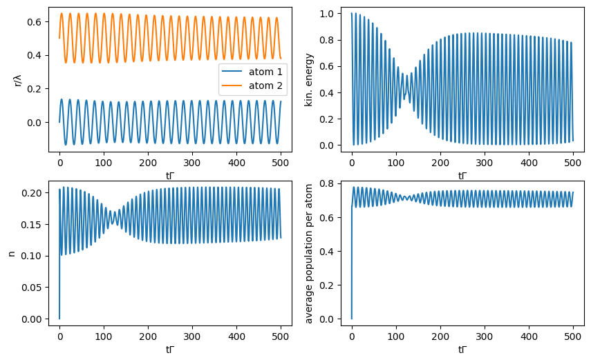

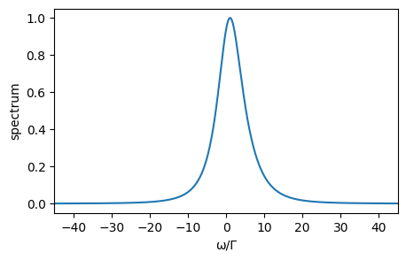
Finally, we calculate the spectrum of the output field. Obviously there is no steady state for our system since the particles always move. Therefore, we calculate the two-time correlation function just for the final state of the cooling process. Due to the semiclassical motion we need to precalculate the positions of the particles to obtain the spectrum, see arXiv:1906.01945 for details.

#calculate semiclassical spectrumT_spec = [0:0.01:50;]t1, ρt1 = semiclassical.master_dynamic(T_spec,ρt[end],f_q,f_cl!; alg=Tsit5())r_spec = [[Float64[] for i=1:N_a]...] #postions of the particles at every timestep#produce continous particle trajectories for further calculationsr_spline = []for it=1:N_a    r_spec[it] = [real(ρt1.classical[it]) for ρt1=ρt1]    push!(r_spline, interpolate((t1,), r_spec[it], Gridded(Linear())))endfunction Ht(t,rho)    u = [r_spline[it](t) for it=1:N_a]    H_int = g*sum(cos.(u[1:N_a]*k).*spa_plus_smad)    H = H0 + H_int    return H, J, Jd, ratesendaρ0 = a*ρt[end].quantumτ, aρt = timeevolution.master_dynamic(T_spec,aρ0,Ht; alg=Tsit5())corr = expect(ad, aρt)ω, spec = timecorrelations.correlation2spectrum(τ, corr)spec_0 = spec .- minimum(spec) #set spectrum minimum to 0spec_0_norm = spec_0./maximum(spec_0)

figure(figsize=(5, 3))plot(ω/Γ, spec_0_norm)xlabel("ω/Γ")ylabel("spectrum")xlim(xmin=-45, xmax=45)