This notebook can be found on github

Pumped cavity

using QuantumOpticsusing PyPlot

Define parameters

using Random; Random.seed!(0)η = 0.9 # Pumping strengthκ = 1 # Decay rateNcutoff = 20 # Maximum photon numberT = [0:0.1:10;]

Create Fock basis and all operators

basis = FockBasis(20)a = destroy(basis)at = create(basis)n = number(basis)H = η*(a+at)J = [sqrt(κ)*a]

Define initial state

Ψ₀ = fockstate(basis, 10)ρ₀ = Ψ₀ ⊗ dagger(Ψ₀)

Time evolution according to master equation

tout, ρt_master = timeevolution.master(T, ρ₀, H, J)

Three different monte carlo trajectories

tout_example1, Ψt_example1 = timeevolution.mcwf(T, Ψ₀, H, J; seed=UInt(1),                                        display_beforeevent=true,                                        display_afterevent=true)tout_example2, Ψt_example2 = timeevolution.mcwf(T, Ψ₀, H, J; seed=UInt(2),                                        display_beforeevent=true,                                        display_afterevent=true)tout_example3, Ψt_example3 = timeevolution.mcwf(T, Ψ₀, H, J; seed=UInt(3),                                        display_beforeevent=true,                                        display_afterevent=true)

Calculate expectation values $\langle n(t) \rangle$ by averaging single monte carlo trajectory expectation values

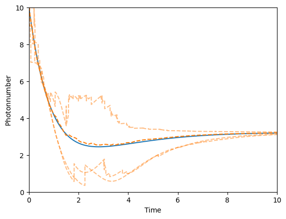
Ntrajectories = 50n_average = zeros(Float64, length(T))function fout(t::Float64, psi::Ket)    i = findfirst(isequal(t), T)    n_average[i] += real(expect(n, psi)/norm(psi)^2)endfor i=1:Ntrajectories    timeevolution.mcwf(T, Ψ₀, H, J; fout=fout)endn_average /= Ntrajectories

Plot the result $\langle n(t) \rangle$ for the master equation, three different single MCWF trajectories and the average of many MCWF trajectories

plot(T, real(expect(n, ρt_master)))plot(T, n_average, "--")plot(tout_example1, real(expect(n, Ψt_example1)), "C1--", alpha=0.5)plot(tout_example2, real(expect(n, Ψt_example2)), "C1--", alpha=0.5)plot(tout_example3, real(expect(n, Ψt_example3)), "C1--", alpha=0.5)xlim(0, 10)ylim(0, 10)xlabel(L"\mathrm{Time}")ylabel(L"\mathrm{Photon number}")