This notebook can be found on github

Ramsey spectroscopy of two-level atom ensemble

Consider an ensemble of two-level atoms (spin-1/2 particles) with transition frequency $\omega_{a}$ subject to decay. The Hamiltonian of the system is

$H_{at} = \frac{\Delta}{2}\sum_i\sigma_i^z,$

where $\Delta = \omega_a - \omega_l$ and $\omega_l$ is a reference frequency. We describe the decay with rate $\gamma$ via the Lindblad term

$\mathcal{L}[\rho] = \frac{\gamma}{2}\sum_i\left(2\sigma_i^-\rho\sigma_i^+ - \sigma_i^+\sigma_i^-\rho - \rho\sigma_i^+\sigma_i^-\right).$

Say we want to perform a Ramsey interferometry scheme on this ensemble. This is done in three stages:

A laser pulse (laser frequency $\omega_l$) with amplitude $\eta$ is applied for a time $T$ such that $\eta T=\frac{\pi}{4}$ ($\pi/2$-pulse).
The ensemble is left to evolve freely under the Hamiltonian $H_{at}$ and the Liouvillian $\mathcal{L}[\rho]$.
Finally, another $\pi/2$-pulse is applied and the total population inversion $\sum_i\langle\sigma_i^z\rangle$ is measured.

using QuantumOpticsusing PyPlot

N = 2 # Atom numberγ = 0.1 # Decay rateΔ = 0.05 # Detuningη = 15.0 # Pulse strengthT = π/4η # Length for pulseTsteps = 101Tlist = collect(range(0, stop=T, length=Tsteps))τ = γ == 0 ? 1.0 : 0.5/γ # Length of free time evolution; 1.0 if γ=0, else 0.5/γτsteps = 201τlist = collect(range(0, stop=τ, length=τsteps))b_atom = SpinBasis(1//2)b_coll = tensor([b_atom for i=1:N]...)

# Single atom operatorssm(i) = embed(b_coll, i, sigmam(b_atom))sp(i) = embed(b_coll, i, sigmap(b_atom))sz(i) = embed(b_coll, i, sigmaz(b_atom))# Collective operatorsSx = 0.5*sum(sm.(1:N) + sp.(1:N))Sy = 0.5im*sum(sm.(1:N) - sp.(1:N))Sz = 0.5*sum(sz.(1:N))

H_at = Δ*Sz

The Hamiltonian of the driving laser is $H_l = \eta\sum_i\left(\sigma_i^- + \sigma_i^+\right)=2\eta S_x.$

H_l = 2η*Sx;J = [sm(i) for i=1:N]rates = [γ for i=1:N]

ψ₀ = tensor([spindown(b_atom) for i=1:N]...)

A convenient way to illustrate a quantum state is the so-called Bloch sphere, which can be generalized to a collection of atoms. The collective Bloch vector is defined by

$\vec{B} = \left(\langle S_x\rangle, \langle S_y\rangle, \langle S_z\rangle\right)^\mathrm{T}$.

We define a function to calculate this vector.

bloch(ρ) = [real(expect(s, ρ)) for s=[Sx, Sy, Sz]]

The Bloch vector of the initial state (all atoms in the ground state) then points downwards on the sphere.

# Plot a circle with x and y labels (the Bloch sphere from different sides)function plot_circle(x, y)    ϕ = collect(range(0, stop=2π, length=201))    plot(cos.(ϕ), sin.(ϕ))        # Label circle axes    text(0.9, 0.05, x)    text(0.05, 0.9, y)        # Draw axes    plot([0, 0], [0, 1], "k", lw=0.5)    plot([0, 1], [0, 0], "k", lw=0.5)end

bloch0 = bloch(dm(ψ₀))fig = figure(figsize=(9, 3))ax1 = subplot(131)plot_circle("x","y")plot([0, bloch0[1]], [0, bloch0[2]], lw=3)ax1.axis("off")ax2 = subplot(132)plot_circle("x", "z")plot([0, bloch0[1]], [0, bloch0[3]], lw=3)ax2.axis("off")ax3 = subplot(133)plot_circle("y", "z")plot([0, bloch0[2]], [0, bloch0[3]], lw=3)ax3.axis("off")tight_layout()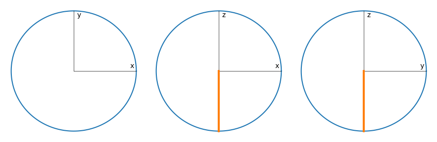

png

1) First $\pi/2$-pulse

Tout, ρT = timeevolution.master(Tlist, ψ₀, H_at + H_l, J; rates=rates)inv_π2 = sum([real(expect(sz(i), ρT)) for i=1:N])ρπ2 = ρT[end]; # State after first π/2-pulse

bloch_π2 = bloch(ρπ2)fig = figure(figsize=(9, 3))ax1 = subplot(131)plot_circle("x","y")plot([0, bloch_π2[1]], [0, bloch_π2[2]], lw=3)ax1.axis("off")ax2 = subplot(132)plot_circle("x", "z")plot([0, bloch_π2[1]], [0, bloch_π2[3]], lw=3)ax2.axis("off")ax3 = subplot(133)plot_circle("y", "z")plot([0, bloch_π2[2]], [0, bloch_π2[3]], lw=3)ax3.axis("off")tight_layout()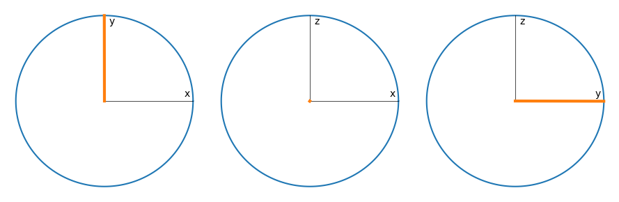

png

2) Free time evolution

τout, ρτ = timeevolution.master(τlist, ρπ2, H_at, J; rates=rates);ρm = ρτ[end]; # State after free time evolution

bloch_m = bloch(ρm)fig = figure(figsize=(9, 3))ax1 = subplot(131)plot_circle("x","y")plot([0, bloch_m[1]], [0, bloch_m[2]], lw=3)ax1.axis("off")ax2 = subplot(132)plot_circle("x", "z")plot([0, bloch_m[1]], [0, bloch_m[3]], lw=3)ax2.axis("off")ax3 = subplot(133)plot_circle("y", "z")plot([0, bloch_m[2]], [0, bloch_m[3]], lw=3)ax3.axis("off")tight_layout()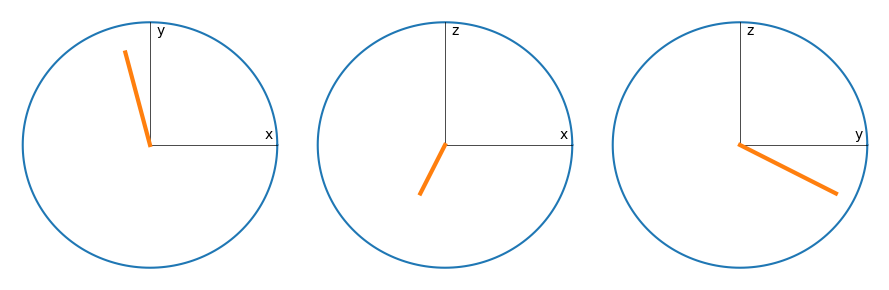

png

3) Second $\pi$-2 pulse

Tout, ρT = timeevolution.master(Tlist, ρm, H_at + H_l, J; rates=rates)ρπ = ρT[end]; # Final state after second π/2-pulse

bloch_π = bloch(ρπ)fig = figure(figsize=(9, 3))ax1 = subplot(131)plot_circle("x","y")plot([0, bloch_π[1]], [0, bloch_π[2]], lw=3)ax1.axis("off")ax2 = subplot(132)plot_circle("x", "z")plot([0, bloch_π[1]], [0, bloch_π[3]], lw=3)ax2.axis("off")ax3 = subplot(133)plot_circle("y", "z")plot([0, bloch_π[2]], [0, bloch_π[3]], lw=3)ax3.axis("off")tight_layout()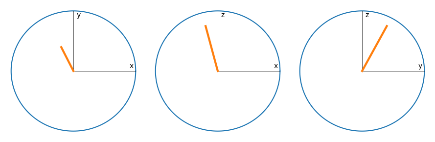

png

As you can see, for the chosen parameters we end up in a state near the fully inverted one, with an inversion of

print(bloch_π[3])

0.7475443402325713

Ramsey fringes

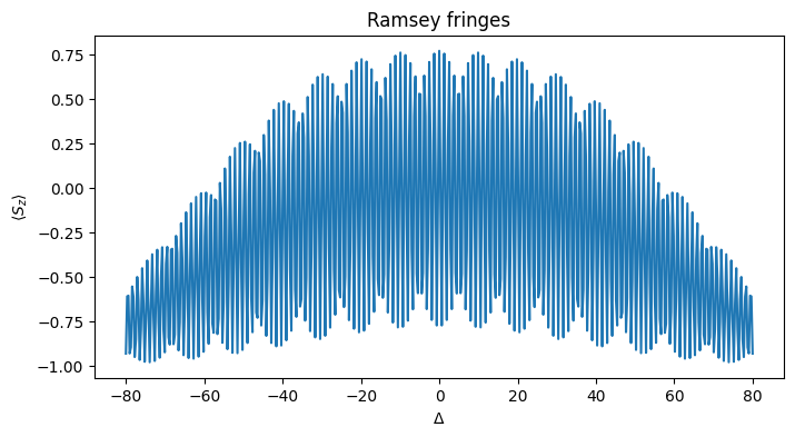
Now, in order to obtain the famous Ramsey fringes, we have to scan over the laser frequency, i.e. the detuning. To this end, we need to do the entire above procedure but for different detunings.

Let's write a function for the above procedure but allowing for different detunings that returns the final population inversion.

function ramsey(Δ)    H_at = Δ*Sz    Tout, ρ1 = timeevolution.master(Tlist, ψ₀, H_at + H_l, J; rates=rates) # First π/2-pulse    τout, ρτ = timeevolution.master(τlist, ρ1[end], H_at, J; rates=rates) # Free time evolution    Tout, ρ2 = timeevolution.master(Tlist, ρτ[end], H_at + H_l, J; rates=rates) # Second π/2-pulse    real(expect(Sz, ρ2[end])) # Return resulting final inversionend

Δ_ls = collect(range(-80, stop=80, length=501)) # List of detuningsSz_exp = ramsey.(Δ_ls)figure(figsize=(8, 4))plot(Δ_ls, Sz_exp)ylabel(L"$\langle S_z\rangle$")xlabel(L"$\Delta$")title("Ramsey fringes")

png