This notebook can be found on github

Heat-pumped three-level maser

Consider a three-level atom that interacts with two heat baths at temperatures $T_\mathrm{c}$ and $T_\mathrm{h}$, respectively, and a single cavity field mode. The cavity mode is further coupled to an environment at temperature $T_\mathrm{env}$.

The atomic transition $|1\rangle \leftrightarrow |3\rangle$ at frequency $\omega_\mathrm{h}:=\omega_3-\omega_1$ is coupled to the hot bath, the atomic transition $|2\rangle \leftrightarrow |3\rangle$ at frequency $\omega_\mathrm{c}:=\omega_3-\omega_2$ is coupled to the cold bath and the atomic transition $|1\rangle \leftrightarrow |2\rangle$ at frequency $\omega_\mathrm{f}:=\omega_2-\omega_1$ (the lasing transition) is coupled to the cavity mode.

The Hamiltonian

$H=H_\mathrm{free}+H_\mathrm{int}$

consists of the "free" atomic and cavity Hamiltonian

$H_\mathrm{free}=\hbar\omega_1 |1\rangle\langle 1|+\hbar\omega_2 |2\rangle\langle 2|+\hbar\omega_3 |3\rangle\langle 3|+\hbar\omega_\mathrm{f}a^\dagger a$

and the Jaynes-Cummings interaction

$H_\mathrm{int}=\hbar g\left(\sigma_{12}a^\dagger+\sigma_{21} a\right).$

The interaction with the various environmental heat baths is described by the Liouvillian

$\mathcal{L}\rho = \frac{\gamma_\mathrm{h}}{2}[\bar{n}(\omega_\mathrm{h},T_\mathrm{h})+1] \mathcal{D}[\sigma_{13}] + \frac{\gamma_\mathrm{h}}{2}\bar{n}(\omega_\mathrm{h},T_\mathrm{h}) \mathcal{D}[\sigma_{31}]\\ \quad + \frac{\gamma_\mathrm{c}}{2}[\bar{n}(\omega_\mathrm{c},T_\mathrm{c})+1] \mathcal{D}[\sigma_{23}] + \frac{\gamma_\mathrm{c}}{2}\bar{n}(\omega_\mathrm{c},T_\mathrm{c}) \mathcal{D}[\sigma_{32}]\\ \quad + \kappa[\bar{n}(\omega_\mathrm{f},T_\mathrm{env})+1] \mathcal{D}[a] + \kappa\bar{n}(\omega_\mathrm{f},T_\mathrm{env}) \mathcal{D}[a^\dagger],$

where the dissipator is defined as $\mathcal{D}[A]:= 2A\rho A^\dagger - A^\dagger A \rho -\rho A^\dagger A$.

The time evolution of the joint atom-field state is then given by the master equation

$\dot{\rho}(t) = \frac{1}{i\hbar}[H,\rho] + \mathcal{L}\rho.$

using QuantumOpticsusing PyPlotusing LinearAlgebra

const nph=50     # cavity mode photon cutoffconst Th=100.    # temperature of the hot bathconst Tc=20.     # temperature of the cold bathconst Tenv=0.    # environment temperature for the cavityconst omega1=0.const omega2=30.const omega3=150.const omegaf=omega2-omega1  # cavity frequency (lasing frequency)const omegah=omega3-omega1  # frequency of the atomic transition that is coupled to the hot bathconst omegac=omega3-omega2  # frequency of the atomic transition that is coupled to the cold bathconst g=5.const kappa=0.1const gammah=40.const gammac=40.const tmax=50.const dt=.1const tvec=[0.:dt:tmax;]        # output times for expectation values (high resolution)const dtrho=10.const trhovec=[0.:dtrho:tmax;]; # output times for the density matrix (low resolution)

const ba=NLevelBasis(3)const bf=FockBasis(nph)const b_comp=ba⊗bfconst psi1=nlevelstate(ba,1)const psi2=nlevelstate(ba,2)const psi3=nlevelstate(ba,3)const proj1=projector(psi1)⊗one(bf)const proj2=projector(psi2)⊗one(bf)const proj3=projector(psi3)⊗one(bf)const sigma13=transition(ba,1,3)⊗one(bf)const sigma23=transition(ba,2,3)⊗one(bf)const sigma12=transition(ba,1,2)⊗one(bf)const a=one(ba)⊗destroy(bf)

const Hfree=omega1*proj1+omega2*proj2+omega3*proj3+omegaf*dagger(a)*aconst Hint=g*(sigma12*dagger(a)+a*dagger(sigma12))const H=Hfree+Hint

const R=Array{Float64}(undef,6)nbar(omega::Float64,T::Float64)=(exp(omega/T)-1)^(-1) # hbar=k_B=1R[1]=gammah*(nbar(omegah,Th)+1)R[2]=gammah* nbar(omegah,Th)R[3]=gammac*(nbar(omegac,Tc)+1)R[4]=gammac* nbar(omegac,Tc)R[5]=2*kappa*(nbar(omegaf,Tenv)+1)R[6]=2*kappa* nbar(omegaf,Tenv)const J=[sqrt(R[1])*sigma13,sqrt(R[2])*dagger(sigma13),         sqrt(R[3])*sigma23,sqrt(R[4])*dagger(sigma23),         sqrt(R[5])*a,sqrt(R[6])*dagger(a)]

const trho=Array{Float64}(undef,length(trhovec))const rho=[DenseOperator(b_comp) for k=1:length(trhovec)]# This dictionary contains the operators whose expectation values should be # computed with high resolution during the time evolutionconst operators=Dict(:adagger_a=>a'*a,                     :adagger_adagger_a_a=>a'*a'*a*a,                     :population1=>proj1,                     :population2=>proj2,                     :population3=>proj3)function compute_expvalues(τ,ρ)    index=findfirst(isapprox.(τ,trhovec)) # The comparison of floats is problematic        if !isnothing(index) # save ρ if τ is contained in throvec            trho[index]=τ            rho[index]=copy(ρ)        end    return Dict{Symbol,ComplexF64}(key=>expect(value,ρ) for (key,value) in operators)end

const r0=dm(psi1)⊗dm(fockstate(bf,0))normalize!(r0)    t,expvalues=timeevolution.master(tvec,r0,H,J;fout=compute_expvalues)

g2=real.(getindex.(expvalues,:adagger_adagger_a_a)./getindex.(expvalues,:adagger_a).^2)rhof=[ptrace(r,1) for r in rho]x=[-7.5:0.01:7.5;]qfunc_ss=qfunc(rhof[end],x,x); # steady-state Q function

figure(figsize=[12.8,8.6])subplot(2,2,1)plot(t,real.(getindex.(expvalues,:population1)),label="population of level "*L"|1\rangle")plot(t,real.(getindex.(expvalues,:population2)),label="population of level "*L"|2\rangle")plot(t,real.(getindex.(expvalues,:population3)),label="population of level "*L"|3\rangle")title("atomic populations")xlabel("t")legend()grid()subplot(2,2,2)plot(t,real.(getindex.(expvalues,:adagger_a)))title("photon number")xlabel("t")ylabel(L"\langle a^\dagger a\rangle")grid()subplot(2,2,3)plot(tvec,g2)title(L"g^{(2)}"*" function")xlabel("t")ylabel(L"g^{(2)}(0)")grid()subplot(2,2,4)pcolormesh(x,x,transpose(real(qfunc_ss)),cmap="jet")axis("equal")title(L"Q"*" function at "*L"t="*string(tvec[end]))xlabel(L"$\mathrm{Re}\,\alpha$")ylabel(L"$\mathrm{Im}\,\alpha$")tight_layout()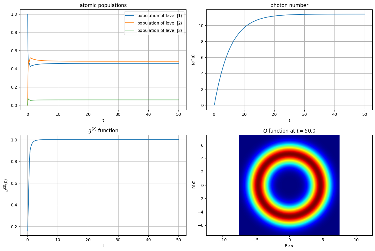

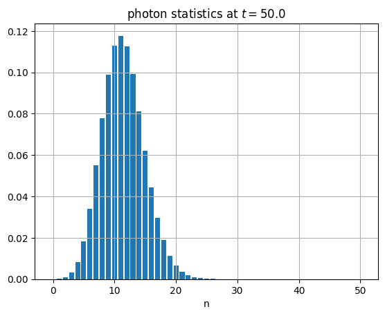
bar([0:nph;],real.(diag(rhof[end].data)))title("photon statistics at "*L"t="*string(tvec[end]))xlabel("n")grid()