Stimulated Emission

We simulate the emission of an atom stimulated by an incident quantum pulse. In particular, how efficiently such stimulated emission occurs into the mode occupied by the incident photons. This system is described in A. Kiilerich, et al., Phys. Rev. Lett. 123, 123604 (2019). The initially excited atom has a decay rate $\Gamma$ and the incident quantum pulse is a single photon in an exponentially decaying mode $u(t) = \sqrt{\Gamma} e^{-\Gamma t/2}$.

We start by loading the packages and defining the symbolic operators and parameters.

using QuantumInputOutputusing SecondQuantizedAlgebrausing QuantumOpticsusing QuantumOpticsBase: daggerusing Plotsusing LaTeXStrings

# symbolic Hilbert spaceshu1 = FockSpace(:u1)hc1 = NLevelSpace(:atom1, 2)hv1 = FockSpace(:v1)h = hu1 ⊗ hc1 ⊗ hv1# symbolic operatorsau = Destroy(h, :a_u, 1)σ(i, j) = Transition(h, :σ, i, j, 2)av = Destroy(h, :a_v, 3)# symbolic parameters@variables γ::Real Δ::Real Γ::Real g_v::Real

We use the symbolic operators and parameters to define the SLH triples and cascade them to obtain the Hamiltonian and Lindblad for the system.

G_u = SLH(1, √(Γ)*au, 0) # input cavityG_c = SLH(1, √(γ)*σ(1, 2), Δ*σ(2, 2)) # two-level atomG_v = SLH(1, g_v'*av, 0) # output cavityG_cas = G_u ▷ G_c ▷ G_v

H = G_cas.hamiltonian

Δ * σ₂₂ + (-0.5sqrt(γ)*sqrt(Γ))im * a_u * σ₂₁ + (-0.5g_v*sqrt(Γ))im * a_u * a_v' + (0.5sqrt(γ)*sqrt(Γ))im * a_u' * σ₁₂ + (0.5g_v*sqrt(Γ))im * a_u' * a_v + (-0.5g_v*sqrt(γ))im * σ₁₂ * a_v' + (0.5g_v*sqrt(γ))im * σ₂₁ * a_v

L = G_cas.jump_operator[1] # only one Lindblad in this example

sqrt(Γ) * a_u + sqrt(γ) * σ₁₂ + g_v * a_v

# numerical parameters and functionsγ_ = 1.0Δ_ = 0.0Γ_ = γ_/0.36p_sym = [γ, Δ, Γ]p_num = [γ_, Δ_, Γ_]dict_p = Dict(p_sym .=> p_num)gv_(t) = √(Γ_/(exp(Γ_*t) - 1))dict_p_t = Dict(g_v => gv_)T = [0.001:0.001:1;]*4.0ΔT = T[2] - T[1]

We use the function to_numeric to create the numeric operators and solve the dynamics with the function timeevolution.master_dynamic in QuantumOptics.jl.

# numeric basesbu1 = FockBasis(1)ba1 = NLevelBasis(2)bv1 = FockBasis(2)b = bu1 ⊗ ba1 ⊗ bv1H_QO = to_numeric(H, b; parameter = dict_p, time_parameter = dict_p_t)L_QO = to_numeric(L, b; parameter = dict_p, time_parameter = dict_p_t)function input_output(t, ρ)    H = H_QO(t)    J = [L_QO(t)]    return H, J, dagger.(J)end;# initial stateψ0 = fockstate(bu1, 1) ⊗ nlevelstate(ba1, 2) ⊗ fockstate(bv1, 0)# time evolutiont_, ρt = timeevolution.master_dynamic(T, ψ0, input_output)

To calculate expectation values we create the desired numerical operators.

au_qo = to_numeric(au, b)σ_qo(i, j) = to_numeric(σ(i, j), b)av_qo = to_numeric(av, b)proj_u(n) = embed(b, 1, projector(fockstate(bu1, n)))proj_v(n) = embed(b, 3, projector(fockstate(bv1, n)))popu_u_n1 = real.(expect(proj_u(1), ρt))popu_e = real.(expect(σ_qo(2, 2), ρt))popu_v_n1 = real.(expect(proj_v(1), ρt))popu_v_n2 = real.(expect(proj_v(2), ρt))L0(t) = √(γ_)*σ_qo(1, 2) + √(Γ_)*au_qo + gv_(t)*av_qoI_out = [real(expect(dagger(L0(t_[i]))*L0(t_[i]), ρt[i])) for i = 1:length(t_)]I_out_int = [0.0]for i = 2:length(I_out)    push!(I_out_int, I_out_int[end]+I_out[i]*ΔT)end

p = plot(t_, popu_u_n1; color = :red, label = L"| 1 \rangle_u")plot!(p, t_, popu_e; color = :pink, ls = :dash, label = L"| e \rangle")plot!(p, t_, popu_v_n1; color = :blue, ls = :dash, label = L"| 1 \rangle_v")plot!(p, t_, popu_v_n2; color = :green, label = L"| 2 \rangle_v")plot!(p, t_, I_out_int; color = :black, ls = :dot, label = L"\\int I_{out} dt")plot!(    p;    xlims = (0, 4),    ylims = (0, 1),    xlabel = "time [1/γ]",    ylabel = "population",    legend = :best,    size = (600, 300),)p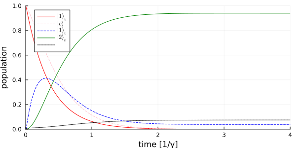

Package versions

These results were obtained using the following versions:

using InteractiveUtilsversioninfo()using PkgPkg.status([    "QuantumInputOutput",    "SecondQuantizedAlgebra",    "QuantumOptics",    "Plots",    "LaTeXStrings",])

Julia Version 1.13.2
Commit 45b6d15e34b (2026-10-14 20:33 UTC)
Build Info:
  Official https://julialang.org release
Platform Info:
  OS: Linux (x86_64-linux-gnu)
  CPU: 4 × Intel(R) Xeon(R) Platinum 8370C CPU @ 2.80GHz
  WORD_SIZE: 64
  LLVM: libLLVM-20.1.8 (ORCJIT, icelake-server)
  GC: Built with stock GC
Threads: 1 default, 0 interactive, 1 GC (on 4 virtual cores)
Environment:
  JULIA_PKG_SERVER_REGISTRY_PREFERENCE = eager
  JULIA_DEBUG = Documenter,Literate
  JULIA_NUM_THREADS = 1
Status `~/work/QuantumInputOutput.jl/QuantumInputOutput.jl/docs/Project.toml`
  [b964fa9f] LaTeXStrings v1.4.1
  [91a5bcdd] Plots v1.41.7
  [18f9eda6] QuantumInputOutput v0.5.3 `~/work/QuantumInputOutput.jl/QuantumInputOutput.jl`
  [6e0679c1] QuantumOptics v1.2.10
⌅ [f7aa4685] SecondQuantizedAlgebra v0.11.0
Info Packages marked with ⌅ have new versions available but compatibility constraints restrict them from upgrading. To see why use `status --outdated`

This page was generated using Literate.jl.