Tutorial

The basic usage is probably best illustrated with a brief example. In the following, we describe the cavity scattering of a single photon. A common procedure is as follows

build the SLH model
translate it to numerical operators
simulate the dynamics
compute the two-time correlation matrix and extract the dominant output mode
simulate the dynamics again with the output mode

1. Setup and symbolic model

We start by defining the symbolic Hilbert space, operators, and parameters. The model is a one-sided cavity with an input mode u, a system mode c, and an output mode v.

using QuantumInputOutputusing SecondQuantizedAlgebrausing QuantumOpticsusing QuantumOpticsBase: daggerusing LinearAlgebrausing Plotsusing LaTeXStrings

hu1 = FockSpace(:u1)hc1 = FockSpace(:c1)hv1 = FockSpace(:v1)h = hu1 ⊗ hc1 ⊗ hv1au = Destroy(h, :a_u, 1)c = Destroy(h, :c, 2)av = Destroy(h, :a_v, 3)@variables g_u::Complex Δ::Real γ::Real g_v::Complex

The SLH triples for the input mode, system cavity, and output mode are then cascaded to obtain the effective Hamiltonian and Lindblad operator.

G_u = SLH(1, g_u * au, 0)G_c = SLH(1, √(γ) * c, Δ * c' * c)G_v = SLH(1, g_v * av, 0)G_cas = ▷(G_u, G_c, G_v)

H = hamiltonian(G_cas)

\[0.5 ~ \mathrm{imag}\left( \mathtt{g_{u}} \right) ~ \sqrt{\gamma} - 0.5 ~ \mathrm{real}\left( \mathtt{g_{u}} \right) ~ \sqrt{\gamma} ~ \mathit{i} a_{\mathrm{u}}c^{\dagger} + 0.5 ~ \mathrm{imag}\left( \mathtt{g_{u}} \right) ~ \mathrm{real}\left( \mathtt{g_{v}} \right) - 0.5 ~ \mathrm{imag}\left( \mathtt{g_{v}} \right) ~ \mathrm{real}\left( \mathtt{g_{u}} \right) + \left( - 0.5 ~ \mathrm{imag}\left( \mathtt{g_{u}} \right) ~ \mathrm{imag}\left( \mathtt{g_{v}} \right) - 0.5 ~ \mathrm{real}\left( \mathtt{g_{u}} \right) ~ \mathrm{real}\left( \mathtt{g_{v}} \right) \right) ~ \mathit{i} a_{\mathrm{u}}a_{\mathrm{v}}^{\dagger} + 0.5 ~ \mathrm{imag}\left( \mathtt{g_{u}} \right) ~ \sqrt{\gamma} + 0.5 ~ \mathrm{real}\left( \mathtt{g_{u}} \right) ~ \sqrt{\gamma} ~ \mathit{i} a_{\mathrm{u}}^{\dagger}c + 0.5 ~ \mathrm{imag}\left( \mathtt{g_{u}} \right) ~ \mathrm{real}\left( \mathtt{g_{v}} \right) - 0.5 ~ \mathrm{imag}\left( \mathtt{g_{v}} \right) ~ \mathrm{real}\left( \mathtt{g_{u}} \right) + \left( 0.5 ~ \mathrm{imag}\left( \mathtt{g_{u}} \right) ~ \mathrm{imag}\left( \mathtt{g_{v}} \right) + 0.5 ~ \mathrm{real}\left( \mathtt{g_{u}} \right) ~ \mathrm{real}\left( \mathtt{g_{v}} \right) \right) ~ \mathit{i} a_{\mathrm{u}}^{\dagger}a_{\mathrm{v}} - 0.5 ~ \mathrm{imag}\left( \mathtt{g_{v}} \right) ~ \sqrt{\gamma} - 0.5 ~ \mathrm{real}\left( \mathtt{g_{v}} \right) ~ \sqrt{\gamma} ~ \mathit{i} ca_{\mathrm{v}}^{\dagger} + \Delta c^{\dagger}c - 0.5 ~ \mathrm{imag}\left( \mathtt{g_{v}} \right) ~ \sqrt{\gamma} + 0.5 ~ \mathrm{real}\left( \mathtt{g_{v}} \right) ~ \sqrt{\gamma} ~ \mathit{i} c^{\dagger}a_{\mathrm{v}}\]

L = jump_operator(G_cas)[1]

\[\mathrm{real}\left( \mathtt{g_{u}} \right) + \mathrm{imag}\left( \mathtt{g_{u}} \right) ~ \mathit{i} a_{\mathrm{u}} + \sqrt{\gamma} c + \mathrm{real}\left( \mathtt{g_{v}} \right) + \mathrm{imag}\left( \mathtt{g_{v}} \right) ~ \mathit{i} a_{\mathrm{v}}\]

2. Numerical parameters and input pulse

We choose numerical parameters and define a Gaussian input pulse u(t) and calculate the corresponding coupling function g_u(t).

γ_ = 1.0Δ_ = 0.0p_sym = [γ, Δ, g_v]p_num = [γ_, Δ_, 0.0] # g_v = 0dict_p = Dict(p_sym .=> p_num)# Gaussian input modeσ = 1/γ_T_end = 12σu1(t) = 1/(sqrt(σ)*π^(1/4)) * exp( -(t - 4σ)^2 / (2*σ^2) )T = [0:0.002:1;]*T_endΔT = T[2] - T[1]gu_t = coupling_input(u1, T)dict_p_t = Dict(g_u => gu_t)

We define the numerical basis and translate the symbolic operators into QuantumOptics.jl objects. If time_parameter are provided, the result becomes a function of time. Since the purpose of the package is to describe pulses, this is the usual case.

bu1 = FockBasis(2)bc1 = FockBasis(2)bv1 = FockBasis(2)b = bu1 ⊗ bc1 ⊗ bv1H_QO = to_numeric(H, b; parameter=dict_p, time_parameter=dict_p_t)L_QO = to_numeric(L, b; parameter=dict_p, time_parameter=dict_p_t)

3. Time evolution

We now solve the master equation. The required callback for timeevolution.master_dynamic returns H(t), J(t) and J⁺(t) at each time.

function input_output_1(t, ρ)    Ht = H_QO(t)    J = [L_QO(t)]    return Ht, J, dagger.(J)endψ0 = fockstate(bu1, 1) ⊗ fockstate(bc1, 0) ⊗ fockstate(bv1, 0)t_, ρt = timeevolution.master_dynamic(T, ψ0, input_output_1)

4. Two-time correlation function

To extract the dominant output mode, we compute the two-time correlation matrix $g^{(1)}(t_1,t_2) = \langle L_s^\dagger(t_1) L_s(t_2) \rangle$ and diagonalize it. To this end, we first define the desired numerical operators.

au_qo = to_numeric(au, b)c_qo = to_numeric(c, b)av_qo = to_numeric(av, b)Ls(t) = gu_t(t) * au_qo + √(γ_) * c_qog1_m = correlation_matrix(T, ρt, input_output_1, Ls)

p = heatmap(    T,    T,    real.(g1_m);    c = :inferno,    xlabel = L"\gamma t_2",    ylabel = L"\gamma t_1",    colorbar_title = L"g^{(1)}(t_1,t_2)",    size = (400, 350),)p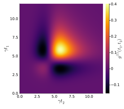

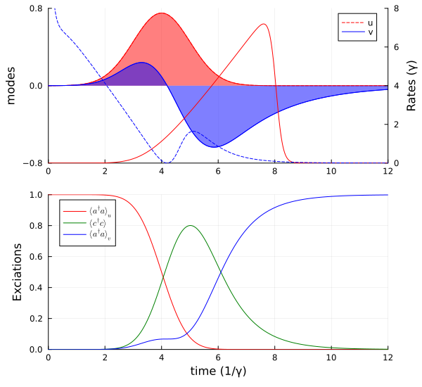
The dominant temporal output mode corresponds to the eigenvector with the largest eigenvalue. With the average photon number in each mode, we can see that the photon is scattered into a single temporal mode.

F = eigen(g1_m)ΔT = T[2] - T[1]n_avg =  round.(real.(F.values)*ΔT; digits=3)modes = F.vectorsv_mode = modes[:, end] / sqrt(ΔT)@show n_avg[end-1:end]

n_avg[var"end" - 1:var"end"] = [0.0, 0.998]

5. Output mode and full dynamics

Finally, we treat the dominant output mode explicitly by providing g_v(t) as a time-dependent parameter, and propagate the system again.

gv_t = coupling_output(v_mode, T)dict_p_t_2 = Dict([g_u, g_v] .=> [gu_t, gv_t])dict_p_2 = Dict([γ, Δ] .=> [γ_, Δ_])H_QO_2 = to_numeric(H, b; parameter=dict_p_2, time_parameter=dict_p_t_2)L_QO_2 = to_numeric(L, b; parameter=dict_p_2, time_parameter=dict_p_t_2)function input_output_2(t, ρ)    Ht = H_QO_2(t)    J = [L_QO_2(t)]    return Ht, J, dagger.(J)end

t_2, ρt_2 = timeevolution.master_dynamic(T, ψ0, input_output_2)n_u_t = real.(expect(au_qo' * au_qo, ρt))n_c_t = real.(expect(c_qo' * c_qo, ρt))n_v_t = real.(expect(av_qo' * av_qo, ρt_2))

Due to the linearity of the system the photon is fully scattered into a single mode.

p1 = plot(T, u1.(T); ls = :dash, label = "u", color = :red)plot!(p1, T, u1.(T); fillrange = 0, fillalpha = 0.5, color = :red, label = "")plot!(p1, T, real.(v_mode); color = :blue, label = "v")plot!(p1, T, real.(v_mode); fillrange = 0, fillalpha = 0.5, color = :blue, label = "")plot!(    p1;    xlims = (0, 12),    ylims = (-0.8, 0.8),    yticks = [-0.8, 0, 0.8],    ylabel = "modes",    legend = :best,)p1r = twinx(p1)plot!(p1r, T, abs2.(gu_t.(T)); color = :red, label = "")plot!(p1r, T[3:end], abs2.(gv_t.(T))[3:end]; color = :blue, ls = :dash, label = "")plot!(p1r; xlims = (0, 12), ylims = (0, 8), ylabel = "Rates (γ)")p2 = plot(T, n_u_t; label = L"\langle a^\dagger a \rangle_u", color = :red)plot!(p2, T, n_c_t; label = L"\langle c^\dagger c \rangle", color = :green)plot!(p2, T, n_v_t; label = L"\langle a^\dagger a \rangle_v", color = :blue)plot!(    p2;    xlims = (0, 12),    ylims = (0, 1),    xlabel = "time (1/γ)",    ylabel = "Exciations",    legend = :best,)plot(p1, p2; layout = (2, 1), size = (600, 550))