Perfect Splitting and Combining of a Two-photon Pulse

In this example, we simulate the perfect splitting of a two-photon pulse into two orthogonal temporal modes with one photon each. We then show the reverse process to combine the two orthogonal photons into a single temporal mode with two photons. The system is described in M. Lund , et al., Phys. Rev. A 107, 023715 (2023).

As usual, we start by loading the packages and defining the symbolic operators and parameters.

using QuantumInputOutputusing SecondQuantizedAlgebrausing QuantumOpticsusing QuantumOpticsBase: daggerusing Plotsusing LaTeXStringsusing LinearAlgebrausing DataInterpolations

# symbolic Hilbert spacehu2 = FockSpace(:u2)hu1 = FockSpace(:u1)hs1 = NLevelSpace(:atom, 2)hv1 = FockSpace(:v1)h = hu2 ⊗ hu1 ⊗ hs1 ⊗ hv1# symbolic operatorsau2 = Destroy(h, :au_2, 1)au1 = Destroy(h, :au_1, 2)σ(i, j) = Transition(h, :σ, i, j, 3)av1 = Destroy(h, :av_2, 4)# symbolic parameters@variables γ::Real Δ::Real gu_1::Number gu_2::Number gv_1::Number

We use the symbolic operators and parameters to define the SLH triples and cascade them to obtain the Hamiltonian and Lindblad for the system.

G_u2 = SLH(1, gu_2'*au2, 0) # input cavity 2G_u1 = SLH(1, gu_1'*au1, 0) # input cavity 1G_a = SLH(1, √(γ)*σ(1, 2), Δ*σ(2, 2)) # scattering atomG_v1 = SLH(1, gv_1'*av1, 0) # output cavity 1G_cas = cascade(G_u2, G_u1, G_a, G_v1)

H = hamiltonian(G_cas)

Δ * σ₂₂ + (-0.5conj(gu_2)*gu_1)im * au_2 * au_1' + (-0.5conj(gu_2)*sqrt(γ))im * au_2 * σ₂₁ + (-0.5conj(gu_2)*gv_1)im * au_2 * av_2' + (0.5conj(gu_1)*gu_2)im * au_2' * au_1 + (0.5gu_2*sqrt(γ))im * au_2' * σ₁₂ + (0.5conj(gv_1)*gu_2)im * au_2' * av_2 + (-0.5conj(gu_1)*sqrt(γ))im * au_1 * σ₂₁ + (-0.5conj(gu_1)*gv_1)im * au_1 * av_2' + (0.5gu_1*sqrt(γ))im * au_1' * σ₁₂ + (0.5conj(gv_1)*gu_1)im * au_1' * av_2 + (-0.5gv_1*sqrt(γ))im * σ₁₂ * av_2' + (0.5conj(gv_1)*sqrt(γ))im * σ₂₁ * av_2

L = jump_operator(G_cas)[1] # only one Lindblad in this example

conj(gu_2) * au_2 + conj(gu_1) * au_1 + sqrt(γ) * σ₁₂ + conj(gv_1) * av_2

Next, the numerical parameters and functions of the system are defined.

γ_ = 1.0Δ_ = 0.0p_sym = [γ, Δ, gu_2, gv_1]p_num = [γ_, Δ_, 0, 0]dict_p = Dict(p_sym .=> p_num)# Gaussian input pulseτ = 0.38;tp = 4/γ_u(t) = 1/(sqrt(τ)*π^(1/4)) * exp(-(t - tp)^2 / (2*τ^2))T = [0:0.002:1;]*20ΔT = T[2] - T[1]gu_ = coupling_input(u, T)dict_p_t = Dict(gu_1 => gu_)

We translate the symbolic expressions to numerical operators and solve the time-dependent master equation with QuantumOptics.jl.

To obtain the output modes we do not use the second input mode and the output mode cavity. However, to keep the example short we include them already from the beginning since they are needed later. To perform time consuming parameter scans one should merely use the necessary Hilbert spaces. In this case, this would correspond to one input cavity and the two-level system. The kwarg operators of the function to_numeric provides a convenient way to use predefined numerical operators, see the example Two-sided Cavity with Atom.

# numeric basesbu2 = FockBasis(2)bu1 = FockBasis(2)bs1 = NLevelBasis(2)bv1 = FockBasis(2)b = bu2 ⊗ bu1 ⊗ bs1 ⊗ bv1;H_QO = to_numeric(H, b; parameter = dict_p, time_parameter = dict_p_t)L_QO = to_numeric(L, b; parameter = dict_p, time_parameter = dict_p_t)function input_output(t, ρ)    H = H_QO(t)    J = [L_QO(t)]    return H, J, dagger.(J)end

# time evolutionψ0 = fockstate(bu2, 0) ⊗ fockstate(bu1, 2) ⊗ nlevelstate(bs1, 1) ⊗ fockstate(bv1, 0)t_, ρt = timeevolution.master_dynamic(T, ψ0, input_output)

Now we analyze the output modes with the two-time autocorrelation function $g^{(1)}(t_1,t_2) = \langle L_s^\dagger(t_1) L_s(t_2) \rangle$.

au1_qo = to_numeric(au1, b)σ_qo(i, j) = to_numeric(σ(i, j), b)Ls(t) = (gu_(t))'*au1_qo + √(γ_)*σ_qo(1, 2)g1_m = correlation_matrix(T, ρt, input_output, Ls);p = heatmap(    T,    T,    real.(g1_m);    c = :inferno,    xlabel = L"\gamma t_2",    ylabel = L"\gamma t_1",    colorbar_title = L"g^{(1)}(t_1,t_2)",    size = (450, 350),)p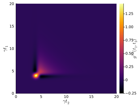

The eigenvalues correspond to the mean photon number $n_i$ in the corresponding temporal eigenvector mode $v_i$. We find two modes with a mean photon number of one.

F = eigen(g1_m)n_avg = real.(F.values)*ΔTmodes = F.vectorsv1_mode = (modes[:, end]) / √(ΔT)v2_mode = (modes[:, end-1]) / √(ΔT)@show n_avg[(end-1):end]

n_avg[var"end" - 1:var"end"] = [0.9959816950397964, 1.0001254065173415]

p = plot(t_, -real.(v1_mode); color = :black, label = "")plot!(p, t_, real.(v2_mode); color = :red, ls = :dash, label = "")plot!(p; xlabel = "time (1/γ)", ylabel = "output mode", size = (500, 350))p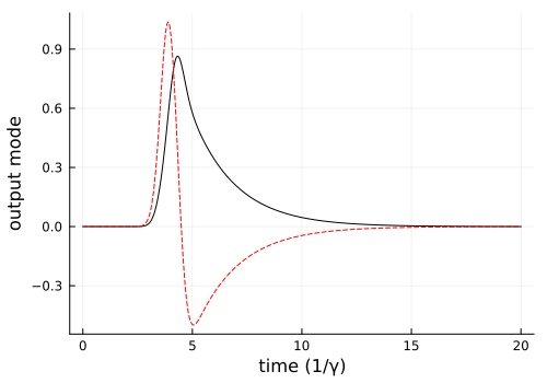

As described in the paper, we can define a rotated basis in which the two modes are not entangled and equally populated by a single photon Fock state. In the following, we define these rotated modes and use them to combine two single photons into a two photon Fock state. The temporal output mode of this two photon Fock state is the same as the previous input mode which separated the two single photons before.

v1_p = 1/√(2) * (v1_mode - v2_mode)v2_p = 1/√(2) * (v1_mode + v2_mode)# new output mode = old input modev1_new(t) = (u(T[end]-t))'# new input modesu1_new = conj.(reverse(v1_p))u2_new = conj.(reverse(v2_p))

The pulse from input cavity $u_2$ is scattered on the cavity $u_1$. This distortion needs to be taken into account for the coupling of $u_2$, which is done with the function effective_input_mode. The coupling of the $u_1$ cavity needs no adaptation, since it directly couples to the two-level system.

gu1_ = coupling_input(u1_new, T)u_new_data = [u1_new, u2_new]u_new_fct = [LinearInterpolation(u, T) for u in u_new_data]# effective u2 mode and corresponding couplingu2_for_gu2 = effective_input_mode(u_new_fct, T, 2)gu2_ = coupling_input(u2_for_gu2, T)# coupling of the output modegv1_ = coupling_output(v1_new, T)# dictionary for the time-dependent functionsg_sym = [gu_1, gu_2, gv_1]g_num = [gu1_, gu2_, gv1_]dict_p_t_out = Dict(g_sym .=> g_num)# dictionary for the constant parametersp_sym_out = [γ, Δ]p_num_out = [γ_, Δ_]dict_p_out = Dict(p_sym_out .=> p_num_out)

The time-dependent couplings are used to define the numeric Hamiltonian and Lindblad term, and then solve the dynamics of the system.

H_QO_2 = to_numeric(H, b; parameter = dict_p_out, time_parameter = dict_p_t_out)L_QO_2 = to_numeric(L, b; parameter = dict_p_out, time_parameter = dict_p_t_out)function input_output_2(t, ρ)    H = H_QO_2(t)    J = [L_QO_2(t)]    return H, J, dagger.(J)end# time evolutionψ0_out = fockstate(bu2, 1) ⊗ fockstate(bu1, 1) ⊗ nlevelstate(bs1, 1) ⊗ fockstate(bv1, 0)t_2, ρt_2 = timeevolution.master_dynamic(T, ψ0_out, input_output_2)

nu1_t_comb = real(expect(au1'*au1, ρt_2))nu2_t_comb = real(expect(au2'*au2, ρt_2))nv1_t_comb = real(expect(av1'*av1, ρt_2))s22_t_comb = real(expect(σ(2, 2), ρt_2))

We can see that the two single photons combine to a two photon Fock-state in one temporal mode.

p = plot(    T,    nu2_t_comb;    color = :red,    ls = :dash,    label = L"\langle a^\dagger a \rangle_{u_2}",)plot!(    p,    T,    nu1_t_comb;    color = :blue,    ls = :dashdot,    label = L"\langle a^\dagger a \rangle_{u_1}",)plot!(p, T, s22_t_comb; color = :black, ls = :dot, label = L"\langle \sigma^{22} \rangle")plot!(    p,    T,    nv1_t_comb;    color = :green,    ls = :solid,    label = L"\langle a^\dagger a \rangle_{v_1}",)plot!(    p;    ylims = (0, 2),    xlims = (10, 18),    xlabel = "time (1/γ)",    ylabel = "Mean Excitation",    legend = :best,    size = (600, 350),)p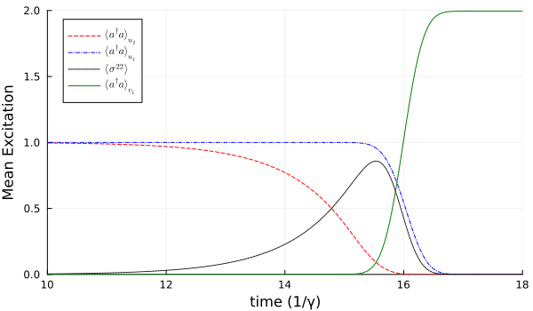

Package versions

These results were obtained using the following versions:

using InteractiveUtilsversioninfo()using PkgPkg.status(    [        "QuantumInputOutput",        "SecondQuantizedAlgebra",        "QuantumOptics",        "Plots",        "DataInterpolations",        "LaTeXStrings",    ],    mode = PKGMODE_MANIFEST,)

Julia Version 1.13.0
Commit d1c37793dd2 (2026-09-09 19:00 UTC)
Build Info:
  Official https://julialang.org release
Platform Info:
  OS: Linux (x86_64-linux-gnu)
  CPU: 4 × AMD EPYC 7763 64-Core Processor
  WORD_SIZE: 64
  LLVM: libLLVM-20.1.8 (ORCJIT, znver3)
  GC: Built with stock GC
Threads: 1 default, 0 interactive, 1 GC (on 4 virtual cores)
Environment:
  JULIA_PKG_SERVER_REGISTRY_PREFERENCE = eager
  JULIA_DEBUG = Documenter,Literate
  JULIA_NUM_THREADS = 1
Status `~/work/QuantumInputOutput.jl/QuantumInputOutput.jl/docs/Manifest.toml`
⌅ [7d9fca2a] Arpack v0.5.3
⌅ [861a8166] Combinatorics v1.0.2
  [d38c429a] Contour v0.6.3
⌅ [82cc6244] DataInterpolations v9.5.0
  [459566f4] DiffEqCallbacks v4.19.4
  [77a26b50] DiffEqNoiseProcess v5.36.4
  [4e289a0a] EnumX v1.0.7
  [c87230d0] FFMPEG v0.4.5
  [7a1cc6ca] FFTW v1.10.0
  [64ca27bc] FindFirstFunctions v3.4.0
⌅ [53c48c17] FixedPointNumbers v0.8.6
  [f6369f11] ForwardDiff v1.4.6
  [069b7b12] FunctionWrappers v1.1.3
  [28b8d3ca] GR v0.73.27
  [42fd0dbc] IterativeSolvers v0.9.4
  [1019f520] JLFzf v0.1.11
  [682c06a0] JSON v1.9.0
  [0b1a1467] KrylovKit v0.10.4
  [b964fa9f] LaTeXStrings v1.4.1
  [23fbe1c1] Latexify v0.16.12
  [7a12625a] LinearMaps v3.11.4
  [442fdcdd] Measures v0.3.3
  [d8a4904e] MutableArithmetics v1.8.1
  [77ba4419] NaNMath v1.1.4
  [e7bfaba1] NumericalIntegration v0.3.4
  [1dea7af3] OrdinaryDiffEq v7.8.1
  [1344f307] OrdinaryDiffEqLowOrderRK v2.2.5
  [ccf2f8ad] PlotThemes v3.3.0
  [995b91a9] PlotUtils v1.5.0
  [91a5bcdd] Plots v1.41.7
  [aea7be01] PrecompileTools v1.3.4
  [08abe8d2] PrettyTables v3.4.8
  [18f9eda6] QuantumInputOutput v0.5.3 `~/work/QuantumInputOutput.jl/QuantumInputOutput.jl`
  [5717a53b] QuantumInterface v0.4.4
  [6e0679c1] QuantumOptics v1.2.10
  [4f57444f] QuantumOpticsBase v0.5.16
  [3cdcf5f2] RecipesBase v1.3.4
  [01d81517] RecipesPipeline v0.6.12
  [731186ca] RecursiveArrayTools v4.5.3
  [189a3867] Reexport v1.2.2
  [05181044] RelocatableFolders v1.0.1
  [ae029012] Requires v1.3.1
  [0bca4576] SciMLBase v3.56.1
  [431bcebd] SciMLPublic v1.3.0
  [6c6a2e73] Scratch v1.3.0
⌅ [f7aa4685] SecondQuantizedAlgebra v0.11.0
  [992d4aef] Showoff v1.1.1
  [276daf66] SpecialFunctions v2.9.0
  [90137ffa] StaticArrays v1.9.22
  [10745b16] Statistics v1.11.5
  [2913bbd2] StatsBase v0.34.13
  [789caeaf] StochasticDiffEq v7.2.0
  [d1185830] SymbolicUtils v4.48.0
  [0c5d862f] Symbolics v7.41.1
  [8ea1fca8] TermInterface v2.0.0
  [1cfade01] UnicodeFun v0.4.1
  [41fe7b60] Unzip v0.2.0
  [2a0f44e3] Base64 v1.11.0
  [ade2ca70] Dates v1.11.0
  [f43a241f] Downloads v1.7.0
  [37e2e46d] LinearAlgebra v1.13.0
  [44cfe95a] Pkg v1.13.0
  [de0858da] Printf v1.11.0
  [3fa0cd96] REPL v1.11.0
  [9a3f8284] Random v1.11.0
  [2f01184e] SparseArrays v1.13.0
  [fa267f1f] TOML v1.0.3
  [cf7118a7] UUIDs v1.11.0
Info Packages marked with ⌅ have new versions available but compatibility constraints restrict them from upgrading. To see why use `status --outdated -m`

This page was generated using Literate.jl.