Photon Number and Mode Entanglement with a Quantum Emitter

We simulate the decay of a three-level Λ emitter through a cavity into two dominant temporal output modes. We identify these modes from the field autocorrelation function, capture them with two virtual output cavities, and visualize the resulting mode populations and the final atom-mode density matrix. This example, reproduces Fig. 4 of A. Kiilerich and K. Molmer, Phys. Rev. A 102, 023717 (2020).

using QuantumInputOutputusing SecondQuantizedAlgebrausing QuantumOpticsusing QuantumOpticsBase: daggerusing Plotsusing LaTeXStringsusing LinearAlgebrausing DataInterpolations

# symbolic Hilbert spacehc = FockSpace(:c)hs = NLevelSpace(:atom, 3)hv1 = FockSpace(:v1)hv2 = FockSpace(:v2)h = hc ⊗ hs ⊗ hv1 ⊗ hv2# symbolic operatorsa = Destroy(h, :a, 1)σ(i, j) = Transition(h, :σ, i, j, 2)av1 = Destroy(h, :a_v1, 3)av2 = Destroy(h, :a_v2, 4)# symbolic parameters@variables γ::Real g::Real ω12::Real g_v1::Number g_v2::Number

The localized system consists of a cavity mode coupled to a three-level Λ emitter. The transition |g₁⟩ ↔ |e⟩ is resonant with the cavity and |g₂⟩ ↔ |e⟩ is detuned by ω₁₂.

H_s = g * (a' * σ(1, 3) + a * σ(3, 1) + a' * σ(2, 3) + a * σ(3, 2)) + ω12 * σ(2, 2)G_s = SLH(1, √(γ) * a, H_s)G_v1 = SLH(1, g_v1' * av1, 0)G_v2 = SLH(1, g_v2' * av2, 0)G = cascade(G_s, G_v1, G_v2)H = hamiltonian(G)L = jump_operator(G)[1]

We use the parameters quoted in the paper and initialize the emitter in the excited state.

γ_ = 1.0g_ = 0.1γ_ω12_ = 0.5γ_T = [0:0.005:1;]*100/γ_ΔT = T[2] - T[1]dict_p_1 = Dict([γ, g, ω12, g_v1, g_v2] .=> [γ_, g_, ω12_, 0.0, 0.0])# numeric bases and operatorsbc = FockBasis(1)bs = NLevelBasis(3)bv1 = FockBasis(1)bv2 = FockBasis(1)b = bc ⊗ bs ⊗ bv1 ⊗ bv2a_qo = destroy(bc) ⊗ one(bs) ⊗ one(bv1) ⊗ one(bv2)σ_qo(i, j) = one(bc) ⊗ transition(bs, i, j) ⊗ one(bv1) ⊗ one(bv2)av1_qo = one(bc) ⊗ one(bs) ⊗ destroy(bv1) ⊗ one(bv2)av2_qo = one(bc) ⊗ one(bs) ⊗ one(bv1) ⊗ destroy(bv2)

We first solve the decay dynamics without explicit output cavities and determine the two dominant temporal output modes from the first-order correlation matrix g⁽¹⁾(t₁, t₂).

H_QO_1 = to_numeric(H, b; parameter = dict_p_1)L_QO_1 = to_numeric(L, b; parameter = dict_p_1)function input_output_1(t, ρ)    J = [L_QO_1]    return H_QO_1, J, dagger.(J)endψ0 = fockstate(bc, 0) ⊗ nlevelstate(bs, 3) ⊗ fockstate(bv1, 0) ⊗ fockstate(bv2, 0)t_1, ρt_1 = timeevolution.master_dynamic(T, ψ0, input_output_1)Ls = √(γ_) * a_qog1_m = correlation_matrix(T, ρt_1, input_output_1, Ls)F = eigen(g1_m)n_avg = real.(F.values) * ΔTv1_mode = F.vectors[:, end] / √(ΔT)v2_mode = F.vectors[:, end-1] / √(ΔT)n1 = n_avg[end]n2 = n_avg[end-1]

After identifying the two modes, we add two cascaded virtual output cavities. The coupling of the second cavity must be corrected for the reshaping caused by the first output cavity, which is done with effective_output_mode.

gv1_t = coupling_output(v1_mode, T)v2_eff = effective_output_mode([v1_mode, v2_mode], T, 2)gv2_t = coupling_output(v2_eff, T)dict_p_2 = Dict([γ, g, ω12] .=> [γ_, g_, ω12_])dict_p_t_2 = Dict(g_v1 => gv1_t, g_v2 => gv2_t)H_QO_2 = to_numeric(H, b; parameter = dict_p_2, time_parameter = dict_p_t_2)L_QO_2 = to_numeric(L, b; parameter = dict_p_2, time_parameter = dict_p_t_2)function input_output_2(t, ρ)    J = [L_QO_2(t)]    return H_QO_2(t), J, dagger.(J)endt_2, ρt_2 = timeevolution.master_dynamic(T, ψ0, input_output_2)

We monitor the excited-state population, the cavity population, and the populations transferred to the two output modes.

P_e_t = real.(expect(σ_qo(3, 3), ρt_2))n_cavity_t = real.(expect(a_qo' * a_qo, ρt_2))n1_t = real.(expect(av1_qo' * av1_qo, ρt_2))n2_t = real.(expect(av2_qo' * av2_qo, ρt_2))

p_a = heatmap(    T,    T,    real.(g1_m);    c = :inferno,    xlabel = L"\gamma t_2",    ylabel = L"\gamma t_1",    colorbar_title = L"g^{(1)}(t_1,t_2)",    xlims = (0, 100),    ylims = (0, 100),    aspect_ratio = 1,)p_b = plot(    T,    real.(v1_mode);    color = :blue,    ls = :dash,    lw = 2,    label = "n₁ = $(round(n1; digits = 2))",)plot!(p_b, T, real.(v2_mode); color = :red, lw = 2, label = "n₂ = $(round(n2; digits = 2))")plot!(p_b; xlabel = L"\gamma t", ylabel = L"\Re[v_i(t)]", legend = :topright)p_c = plot(T, n_cavity_t; color = :green, ls = :dot, lw = 2, label = L"n_\mathrm{cavity}")plot!(p_c, T, P_e_t; color = :black, ls = :dashdot, lw = 2, label = L"P(|e\rangle)")plot!(p_c, T, n1_t; color = :blue, lw = 2, label = L"n_1")plot!(p_c, T, n2_t; color = :red, ls = :dash, lw = 2, label = L"n_2")plot!(    p_c;    xlabel = L"\gamma t",    ylabel = "mean excitation",    ylims = (0, 1),    legend = :topright,)plot(p_a, p_b, p_c, layout = (1, 3), size = (1200, 360))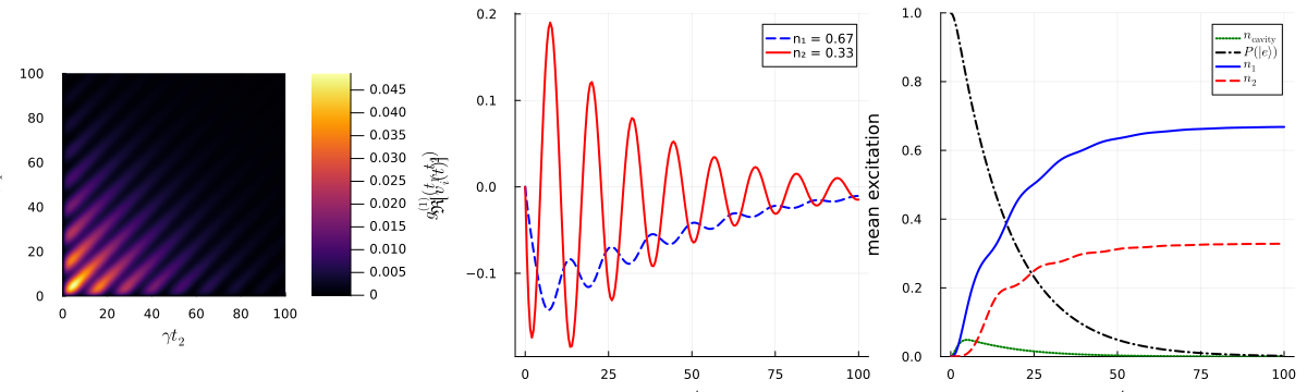

Note that the plotted real part of the output-mode functions are not the same as in the paper due the arbitrary global phase.

Package versions

These results were obtained using the following versions:

using InteractiveUtilsversioninfo()using PkgPkg.status(    [        "QuantumInputOutput",        "SecondQuantizedAlgebra",        "QuantumOptics",        "Plots",        "DataInterpolations",        "LaTeXStrings",    ],    mode = PKGMODE_MANIFEST,)

Julia Version 1.13.0
Commit d1c37793dd2 (2026-09-09 19:00 UTC)
Build Info:
  Official https://julialang.org release
Platform Info:
  OS: Linux (x86_64-linux-gnu)
  CPU: 4 × AMD EPYC 7763 64-Core Processor
  WORD_SIZE: 64
  LLVM: libLLVM-20.1.8 (ORCJIT, znver3)
  GC: Built with stock GC
Threads: 1 default, 0 interactive, 1 GC (on 4 virtual cores)
Environment:
  JULIA_PKG_SERVER_REGISTRY_PREFERENCE = eager
  JULIA_DEBUG = Documenter,Literate
  JULIA_NUM_THREADS = 1
Status `~/work/QuantumInputOutput.jl/QuantumInputOutput.jl/docs/Manifest.toml`
⌅ [7d9fca2a] Arpack v0.5.3
⌅ [861a8166] Combinatorics v1.0.2
  [d38c429a] Contour v0.6.3
⌅ [82cc6244] DataInterpolations v9.5.0
  [459566f4] DiffEqCallbacks v4.19.4
  [77a26b50] DiffEqNoiseProcess v5.36.4
  [4e289a0a] EnumX v1.0.7
  [c87230d0] FFMPEG v0.4.5
  [7a1cc6ca] FFTW v1.10.0
  [64ca27bc] FindFirstFunctions v3.4.0
⌅ [53c48c17] FixedPointNumbers v0.8.6
  [f6369f11] ForwardDiff v1.4.6
  [069b7b12] FunctionWrappers v1.1.3
  [28b8d3ca] GR v0.73.27
  [42fd0dbc] IterativeSolvers v0.9.4
  [1019f520] JLFzf v0.1.11
  [682c06a0] JSON v1.9.0
  [0b1a1467] KrylovKit v0.10.4
  [b964fa9f] LaTeXStrings v1.4.1
  [23fbe1c1] Latexify v0.16.12
  [7a12625a] LinearMaps v3.11.4
  [442fdcdd] Measures v0.3.3
  [d8a4904e] MutableArithmetics v1.8.1
  [77ba4419] NaNMath v1.1.4
  [e7bfaba1] NumericalIntegration v0.3.4
  [1dea7af3] OrdinaryDiffEq v7.8.1
  [1344f307] OrdinaryDiffEqLowOrderRK v2.2.5
  [ccf2f8ad] PlotThemes v3.3.0
  [995b91a9] PlotUtils v1.5.0
  [91a5bcdd] Plots v1.41.7
  [aea7be01] PrecompileTools v1.3.4
  [08abe8d2] PrettyTables v3.4.8
  [18f9eda6] QuantumInputOutput v0.5.3 `~/work/QuantumInputOutput.jl/QuantumInputOutput.jl`
  [5717a53b] QuantumInterface v0.4.4
  [6e0679c1] QuantumOptics v1.2.10
  [4f57444f] QuantumOpticsBase v0.5.16
  [3cdcf5f2] RecipesBase v1.3.4
  [01d81517] RecipesPipeline v0.6.12
  [731186ca] RecursiveArrayTools v4.5.3
  [189a3867] Reexport v1.2.2
  [05181044] RelocatableFolders v1.0.1
  [ae029012] Requires v1.3.1
  [0bca4576] SciMLBase v3.56.1
  [431bcebd] SciMLPublic v1.3.0
  [6c6a2e73] Scratch v1.3.0
⌅ [f7aa4685] SecondQuantizedAlgebra v0.11.0
  [992d4aef] Showoff v1.1.1
  [276daf66] SpecialFunctions v2.9.0
  [90137ffa] StaticArrays v1.9.22
  [10745b16] Statistics v1.11.5
  [2913bbd2] StatsBase v0.34.13
  [789caeaf] StochasticDiffEq v7.2.0
  [d1185830] SymbolicUtils v4.48.0
  [0c5d862f] Symbolics v7.41.1
  [8ea1fca8] TermInterface v2.0.0
  [1cfade01] UnicodeFun v0.4.1
  [41fe7b60] Unzip v0.2.0
  [2a0f44e3] Base64 v1.11.0
  [ade2ca70] Dates v1.11.0
  [f43a241f] Downloads v1.7.0
  [37e2e46d] LinearAlgebra v1.13.0
  [44cfe95a] Pkg v1.13.0
  [de0858da] Printf v1.11.0
  [3fa0cd96] REPL v1.11.0
  [9a3f8284] Random v1.11.0
  [2f01184e] SparseArrays v1.13.0
  [fa267f1f] TOML v1.0.3
  [cf7118a7] UUIDs v1.11.0
Info Packages marked with ⌅ have new versions available but compatibility constraints restrict them from upgrading. To see why use `status --outdated -m`

This page was generated using Literate.jl.