Quantum Pulse Bi-Directional Waveguide

This example mirrors the example Bi-Directional Waveguide but passes numeric operators directly to SLH, circumventing the symbolic derivation part. Furthermore it drives the system with a quantum single-photon pulse via a virtual cavity.

As usual, we start by loading the packages and defining the operators and parameters of the system.

using QuantumInputOutputusing QuantumOpticsusing QuantumOpticsBase: daggerusing Plots

N = 2 # number of quantum dots# numeric Hilbert spacebu = FockBasis(6) # virtual input cavityba = NLevelBasis(2)b_qds = tensor([ba for _ = 1:N]...)b = bu ⊗ b_qds# QD operatorsσ(i, j, k) = embed(b, i+1, transition(ba, j, k))# input mode operatora_u = destroy(bu) ⊗ one(b_qds)# parametersγ = 1.0β = 0.9γRn = fill(γ * β / 2, N)γLn = fill(γ * β / 2, N)γ_add = fill(γ * (1 - β), N)Δn = fill(0.0, N)ϕn = fill(π/10, max(N - 1, 0))# quantum pulse u(t) and virtual cavity coupling g_u(t)σt = 0.8 # pulse witht0 = 4σt  # pulse peakTend = 3t0T = [0:0.005:1;]*TendΔT = T[2]-T[1]u1(t) = 1/(sqrt(σt)*π^(1/4)) * exp(-(t - t0)^2 / (2*σt^2))gu_t = coupling_input(u1, T)

We use the SLH to directly use QuantumOptics.jl operators and functions to the model the system.

G_u = SLH(1, t -> gu_t(t) * a_u, 0*one(b))G_ϕ(i, j) = SLH(exp(1im * ϕn[i]), 0*one(b), 0*one(b))G_R(i) = SLH(1, √(γRn[i]) * σ(i, 1, 2), -Δn[i] * σ(i, 2, 2))G_L(i) = SLH(1, √(γLn[i]) * σ(i, 1, 2), 0*one(b))# Cascade right-moving channelG_R_t = G_u ▷ G_R(1) ▷ G_ϕ(1, 2) ▷ G_R(2)# Cascade left-moving channel (reverse order)G_L_t = G_L(2) ▷ G_ϕ(1, 2) ▷ G_L(1)G_t = G_R_t ⊞ G_L_t

The full Hamiltonian and Lindblad terms are extracted from the final SLH element. Note that as soon as one time-dependent function is involved in a cascade or concatenate, the returned $H$ and $L$ will also be time-dependent.

H = hamiltonian(G_t)L = jump_operator(G_t)L_R = L[1]L_L = L[2]J_add = [√(γ_add[i]) * σ(i, 1, 2) for i = 1:N]function input_output(t, ρ)    Ht = H(t)    J = [L_R(t), L_L(t), J_add...]    return Ht, J, dagger.(J)end

# time evolutionα0 = √(0.1) # √ of total photon numberψ0 = coherentstate(bu, α0) ⊗ tensor([nlevelstate(ba, 1) for _ = 1:N]...)t, ρt = timeevolution.master_dynamic(T, ψ0, input_output)

# transmitted and reflected intensityI_R = zeros(length(t))I_L = zeros(length(t))for (i, ti) in enumerate(t)    LR = L_R(ti)    LL = L_L(ti)    I_R[i] = real(expect(LR' * LR, ρt[i]))    I_L[i] = real(expect(LL' * LL, ρt[i]))end

p = plot(t, I_R; label = "Transmission")plot!(p, t, I_L; label = "Reflection")plot!(p, t, abs2.(α0*u1.(t)); color = :grey, ls = :dash, label = "Input")plot!(    p;    xlabel = "time",    ylabel = "intensity",    legend = :best,    grid = true,    size = (500, 320),)p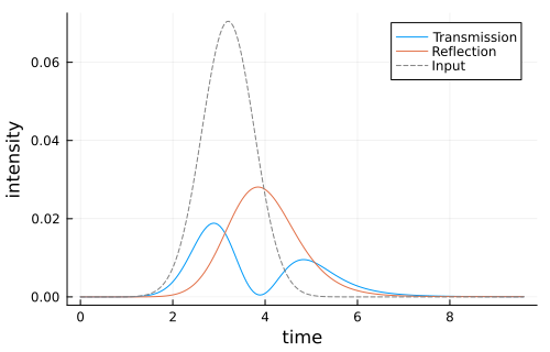

Package versions

These results were obtained using the following versions:

using InteractiveUtilsversioninfo()using PkgPkg.status(["QuantumInputOutput", "QuantumOptics", "Plots"])

Julia Version 1.13.2
Commit 45b6d15e34b (2026-10-14 20:33 UTC)
Build Info:
  Official https://julialang.org release
Platform Info:
  OS: Linux (x86_64-linux-gnu)
  CPU: 4 × Intel(R) Xeon(R) Platinum 8370C CPU @ 2.80GHz
  WORD_SIZE: 64
  LLVM: libLLVM-20.1.8 (ORCJIT, icelake-server)
  GC: Built with stock GC
Threads: 1 default, 0 interactive, 1 GC (on 4 virtual cores)
Environment:
  JULIA_PKG_SERVER_REGISTRY_PREFERENCE = eager
  JULIA_DEBUG = Documenter,Literate
  JULIA_NUM_THREADS = 1
Status `~/work/QuantumInputOutput.jl/QuantumInputOutput.jl/docs/Project.toml`
  [91a5bcdd] Plots v1.41.7
  [18f9eda6] QuantumInputOutput v0.5.3 `~/work/QuantumInputOutput.jl/QuantumInputOutput.jl`
  [6e0679c1] QuantumOptics v1.2.10

This page was generated using Literate.jl.