Input-Output Analysis of Quantum Dot SUPER Excitation

This example analyzes the SUPER excitation scheme for quantum dots with the input-output formalism J. Kerber et al., arXiv (2026). Two red-detuned pulses allow for a close to 100% excitation of a two-level quantum emitter. At the microscopic level, the SUPER mechanism exhibits its nonlinear three-photon Raman-type character, leading to a net photon-number change of −2 in one mode and +1 in the other.

In the first part we describe the dynamics within a cumulant expansion approach for coherent light. We then transform into the interaction-picture of the input and output cavities, which allows us to describe the interaction with large Fock states.

We start by loading the needed packages and specifying the model.

using QuantumInputOutput
using SecondQuantizedAlgebra
using QuantumCumulants
using ModelingToolkitBase
using OrdinaryDiffEq
using QuantumOptics
using Plots
using LaTeXStrings
sol_values(sol, op, eqs) = get_solution(sol, op, eqs).(sol.t)

# Hilbert spaces
hu2 = FockSpace(:u2) # virtual input cavity (u2)
hu1 = FockSpace(:u1) # virtual input cavity (u1)
hs1 = NLevelSpace(:atom, 2) # TLS
hv1 = FockSpace(:v1) # virtual output cavity (v1)
hv2 = FockSpace(:v2) # virtual output cavity (v2)
h = tensor(hu2, hu1, hs1, hv1, hv2)

# Operators
au2 = Destroy(h, :a_u2, 1)
au1 = Destroy(h, :a_u1, 2)
s(i, j) = Transition(h, :s, i, j)
av1 = Destroy(h, :a_v1, 4)
av2 = Destroy(h, :a_v2, 5)

# Symbolic parameters: decay rate and virtual cavity couplings
@variables γ::Real gu1::Number gu2::Number gv1::Number gv2::Number
@independent_variables t # Symbolic time variable

# SLH triplets
G_u2 = SLH(1, gu2'*au2, 0) # input cavity 2
G_u1 = SLH(1, gu1'*au1, 0) # input cavity 1
G_2lvl = SLH(1, √(γ)*s(1, 2), 0) # 2-level system
G_v1 = SLH(1, gv1'*av1, 0) # output cavity 1
G_v2 = SLH(1, gv2'*av2, 0) # output cavity 2

# cascade SLH triplets
G_cas = ▷(G_u2, G_u1, G_2lvl, G_v1, G_v2)

# Hamiltonian and jump operator
Hcas = hamiltonian(G_cas)
Lcas = jump_operator(G_cas)[1]
Lcasd = adjoint(Lcas)

To deal with time-dependent functions in QuantumCumulants.jl, we need to register them.

# Time-dependent couplings
@register_symbolic gu1_t(t)
@register_symbolic gu2_t(t)
@register_symbolic gv1_t(t)
@register_symbolic gv2_t(t)

g_ls = [gu2, gu1, gv1, gv2]
gt_ls = [gu2_t(t), gu1_t(t), gv1_t(t), gv2_t(t)]
dict_gt = Dict(g_ls .=> gt_ls)

# Insert time-dependence
Hcas_t = substitute(Hcas, dict_gt)
Lcas_t = substitute(Lcas, dict_gt)
Lcasd_t = substitute(Lcasd, dict_gt)

We calculate the coupling for the input and output cavities. The modified couplings of the second input and output modes are obtained with the function effective_input_mode and effective_output_mode, respectively. Due to the fast oscillations, the tolerance of the numeric solver needs to be improved. The parameters are taken from T. K. Bracht et al., PRX Quantum 2, 040354 (2021).

# Time grid
dt = 1e-4
Tend = 12*2
T = [dt:dt:Tend;]

# Numerical pulse parameters in THz and ps
γ_ = 1e-2 # TLS decay rate
Δ1_ = -2π*1.934 # detuning pulse 1
Δ2_ = -2π*4.634 # detuning pulse 2
Α1_ = 22.65π # pulse area 1
Α2_ = 19.29π # pulse area 2
σ1_ = 2.4 # temporal FWHM pulse 1
σ2_ = 3.04 # temporal FWHM pulse 2
τ1_ = 0.0 + 12 # time shift pulse 1
τ2_ = -0.73 + 12 # time shift pulse 2

# Normalized input modes
u1(t_) = 1/(√(σ1_)*π^(1/4)) * exp(-(t_ - τ1_)^2 / (2*σ1_^2)) * exp(-1im*Δ1_*t_)
u2(t_) = 1/(√(σ2_)*π^(1/4)) * exp(-(t_ - τ2_)^2 / (2*σ2_^2)) * exp(-1im*Δ2_*t_)

# Coupling functions
gu1_t_ = coupling_input(u1, T)
gu1_t(t) = gu1_t_(t)
gv1_t_ = coupling_output(u1, T)
gv1_t(t) = gv1_t_(t)

# Cascade-modified couplings (effective modes)
abstol = 1e-10
reltol = 1e-10
u_fcts = [u1, u2]
u2_eff = effective_input_mode(u_fcts, T, 2; abstol, reltol)
gu2_t_ = coupling_input(u2_eff, T)
gu2_t(t) = gu2_t_(t)

v_fcts = [u1, u2] # output modes = input modes
v2_eff = effective_output_mode(v_fcts, T, 2; abstol, reltol)
gv2_t_ = coupling_output(v2_eff, T)
gv2_t(t) = gv2_t_(t)

After deriving the mean-field equations we define the initial state, create the ODE problem and solve the dynamics.

# First-order cumulant expansion
order = 1
ops = [au1, au2, s(2, 2), s(2, 1), av1, av2]
eqs = meanfield(ops, Hcas_t, [Lcas_t]; Jdagger = [Lcasd_t], order = order, iv = t)

# Coherent-state amplitudes
α1 = Α1_ / (2*√(2)*π^(1/4)*√(σ1_*γ_)) # field 1
α2 = Α2_ / (2*√(2)*π^(1/4)*√(σ2_*γ_)) # field 2
u0 = [α1, α2, 0, 0, 0, 0.0im]

# Solve ODE system
sys = mtkcompile(System(eqs; name = :sys))
u0_p_map_cas = Dict([unknowns(sys); γ] .=> [u0; γ_])
prob_cas = ODEProblem(sys, u0_p_map_cas, (dt, Tend))
sol = solve(prob_cas, Tsit5(); abstol, reltol)

# Expectation values
t_cas = sol.t # time vector
s22_cas = sol_values(sol, s(2, 2), eqs)
nu1_cas = abs2.(sol_values(sol, au1, eqs))
nu2_cas = abs2.(sol_values(sol, au2, eqs))
nv1_cas = abs2.(sol_values(sol, av1, eqs))
nv2_cas = abs2.(sol_values(sol, av2, eqs))

common = (; xlims = (t_cas[1]-0.01, t_cas[end]))
p1 = plot(
    t_cas,
    real.(s22_cas);
    color = :red,
    label = false,
    ylabel = L"\langle\hat\sigma^{ee}\rangle",
    common...,
)
p2 = plot(
    t_cas,
    nu1_cas;
    color = :blue,
    label = L"\langle \hat{n}_{u_1} \rangle",
    ylabel = L"\langle\hat{n}_i\rangle",
    xticks = ([0, 10, 20], ["", "", ""]),
    yticks = ([0, 5e3, 10e3, 15e3], [L"0", L"5\cdot10^3", L"10\cdot10^3", L"15\cdot10^3"]),
    ylims = (nv1_cas[1]-0.5e3, nu1_cas[1]+0.5e3),
    legend = :left,
    common...,
)
plot!(p2, t_cas, nv1_cas; color = :red, label = L"\langle \hat{n}_{v_1} \rangle")
plot!(
    p2,
    t_cas,
    nu2_cas;
    color = :blue,
    ls = :dash,
    label = L"\langle \hat{n}_{u_2} \rangle",
)
plot!(
    p2,
    t_cas,
    nv2_cas;
    color = :red,
    ls = :dash,
    label = L"\langle \hat{n}_{v_2} \rangle",
)
p3 = plot(
    t_cas,
    nu1_cas .+ nv1_cas .- nu1_cas[1];
    color = :blue,
    label = L"\mathrm{mode~1}",
    ylabel = L"\langle\Delta\hat{n}_i\rangle",
    xlabel = L"\gamma t",
    xticks = ([0, 10, 20], latexstring.([0, 10, 20])),
    yticks = ([-4, -2, 0, 2, 4], latexstring.([-4, -2, 0, 2, 4])),
    legend = :topleft,
    common...,
)
plot!(p3, t_cas, nu2_cas .+ nv2_cas .- nu2_cas[1]; color = :red, label = L"\mathrm{mode~2}")
plot(p1, p2, p3; layout = (3, 1), size = (600, 700))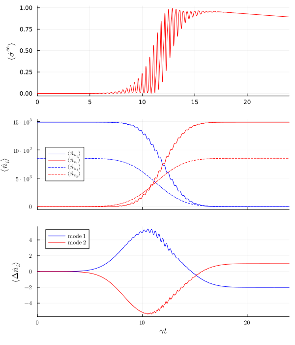

We can see the net photon-number change of −2 in one mode and +1 in the other.

Interaction picture

In the following, we will transform into the interaction picture of the virtual cavities and solve the dynamics.

# Interaction picture: cavity dynamics
H_uv = hamiltonian(▷(G_u2, G_u1, G_v1, G_v2))
H_int_ = simplify(Hcas - H_uv)

M(i, j) = Symbolics.variable(Symbol("M_{$(i)$(j)}"); T = Number)
a0_ls = [au2, au1, av1, av2]
la = length(a0_ls)
a_int_ls = [sum(M(i, j)*a0_ls[j] for j = 1:la) for i = 1:la]
int_dict = Dict(a0_ls .=> a_int_ls)

H_int = substitute(H_int_, int_dict)
L_int = simplify(substitute(Lcas, int_dict))
Ld_int = simplify(substitute(Lcasd, int_dict))

# Coefficient matrix M
Mat = Matrix{Any}(undef, la, la)
for i = 1:la, j = 1:la
    name = Symbol("Ma_$(i)$(j)")
    @eval @register_symbolic $name(t)
    Mat[i, j] = getfield(mod, name)(t)
end
Mat_ls = [Mat[i, j] for i = 1:la for j = 1:la]
M_ls = [M(i, j) for i = 1:la for j = 1:la]

# Time-evolution of the matrix M(t)
A_uv = coupling_matrix((gu2_t_, gu1_t_, gv1_t_, gv2_t_))
M_t = solve_mode_evolution(A_uv, T)

for i = 1:la, j = 1:la
    fname = Symbol("Ma_$(i)$(j)")
    @eval begin
        $fname(t) = M_t(t)[$i, $j]
    end
end
dict_Mt = Dict(M_ls .=> Mat_ls)
dict_gt_Mt = merge(dict_gt, dict_Mt)

H_int_t = substitute(H_int, dict_gt_Mt)
L_int_t = substitute(L_int, dict_gt_Mt)
Ld_int_t = substitute(Ld_int, dict_gt_Mt)

eqs_int = meanfield(ops, H_int_t, [L_int_t]; Jdagger = [Ld_int_t], order = order, iv = t);

# Solve ODE system in interaction picture
sys_int = mtkcompile(System(eqs_int; name = :sysI))
u0_p_map_int = Dict([unknowns(sys_int); γ] .=> [u0; γ_])
prob_int = ODEProblem(sys_int, u0_p_map_int, (dt, Tend))
sol_int = solve(prob_int, Tsit5(); abstol, reltol)

# Expectation values
t_int = sol_int.t
s22_int = real.(sol_values(sol_int, s(2, 2), eqs_int))
nu1_int = abs2.(sol_values(sol_int, au1, eqs_int))
nu2_int = abs2.(sol_values(sol_int, au2, eqs_int))
nv1_int = abs2.(sol_values(sol_int, av1, eqs_int))
nv2_int = abs2.(sol_values(sol_int, av2, eqs_int))

pl4 = plot(
    t_int,
    nu1_int .- nu1_int[1];
    color = :blue,
    label = L"\mathrm{mode~1~(int.)}",
    ylabel = L"\langle\Delta\hat{n}_i\rangle",
    xlabel = L"\gamma t",
    xlims = (t_int[1]-0.01, t_int[end]),
    yticks = ([-2, -1, 0, 1], latexstring.([-2, -1, 0, 1])),
    legend = :right,
    size = (500, 350),
)
plot!(pl4, t_int, nu2_int .- nu2_int[1]; color = :red, label = L"\mathrm{mode~2~(int.)}")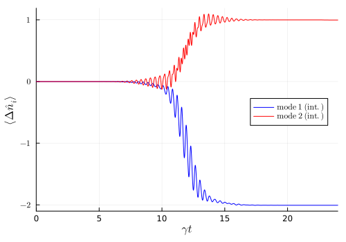

In the interaction picture we can directly observe the photon number change of -2 in one mode and +1 in the other.

Fock state input

Let us now compare the dynamics for coherent input pulses with the case of incident non-classical photon number eigenstates (Fock states), where we choose states with the same mean photon numbers as for the coherent pulses. Since in the atom-field interaction only a few photons are exchanged, the quantum states of the excitation pulses are only changed by a couple of photons, we only need to keep a couple of nearby Fock states in the computational basis.

We define the basis of the system and create the dictionary for the time-dependent variables to translate the Hamiltonian and Lindblad operator to a QuantumOptics.jl operator.

n1_fock = round(Int, abs2(α1))
n2_fock = round(Int, abs2(α2))

bu1 = FockBasis(n1_fock+2, n1_fock-6)
bu2 = FockBasis(n2_fock+3, n2_fock-3)
bs1 = NLevelBasis(2)
bv1 = FockBasis(1)
bv2 = FockBasis(1)
b = tensor([bu2, bu1, bs1, bv1, bv2]...)

g_t_ls = [gu2_t_, gu1_t_, gv1_t_, gv2_t_]
M_t_ls = [t -> M_t(t)[i, j] for i = 1:la for j = 1:la]
dict_fock = Dict([g_ls; M_ls] .=> [g_t_ls; M_t_ls])

H_int_fock = to_numeric(H_int, b; parameter = Dict(γ=>γ_), time_parameter = dict_fock)
L_int_fock = to_numeric(L_int, b; parameter = Dict(γ=>γ_), time_parameter = dict_fock)

TimeDependentSum(dim=504x504)
  basis: [Fock(cutoff=8523, offset=8517) ⊗ Fock(cutoff=14881, offset=14873) ⊗ NLevel(N=2) ⊗ Fock(cutoff=1) ⊗ Fock(cutoff=1)]

To solve the dynamics, we create the time-dependent function for the open quantum system and define the initial state.

function input_output(t, ρ)
    Ht = H_int_fock(t)
    J = [L_int_fock(t)]
    return Ht, J, QuantumOptics.dagger.(J)
end

# initial state
ψu2 = fockstate(bu2, n2_fock)
ψu1 = fockstate(bu1, n1_fock)
ψs1 = nlevelstate(bs1, 1)
ψv1 = fockstate(bv1, 0)
ψv2 = fockstate(bv2, 0)
ψ0 = tensor(ψu2, ψu1, ψs1, ψv1, ψv2)

T_fock = [0:0.001:1;]*T[end]
# t_fock, ρt_fock = timeevolution.master_dynamic(T_fock, ψ0, input_output; abstol, reltol)
using Random
t_fock, ρt_fock = timeevolution.mcwf_dynamic(T_fock, ψ0, input_output; abstol, reltol)

Due to the relatively long computation time of timeevolution.master_dynamic, we simulate a single trajectory with timeevolution.mcwf_dynamic.

# Expectation values
s22_fock = real.(expect(s(2, 2), ρt_fock))
nu1_fock = real.(expect(au1'au1, ρt_fock))
nu2_fock = real.(expect(au2'au2, ρt_fock))
nv1_fock = real.(expect(av1'av1, ρt_fock))
nv2_fock = real.(expect(av2'av2, ρt_fock))

common = (; xlims = (t_fock[1]-0.01, t_fock[end]))
p3_1 = plot(
    t_int,
    s22_int;
    color = :blue,
    label = L"\mathrm{coherent state}",
    ylabel = L"\langle\hat\sigma^{ee}\rangle",
    common...,
)
plot!(p3_1, t_fock, s22_fock; color = :red, label = L"\mathrm{Fock state}")
p3_2 = plot(
    t_fock,
    nu1_fock .- nu1_fock[1];
    color = :green,
    label = L"\mathrm{Fock: mode~1}",
    ylabel = L"\langle\Delta\hat{n}_i\rangle",
    xlabel = L"\gamma t",
    xlims = (t_fock[1]-0.01, t_fock[end]),
    yticks = ([-2, -1, 0, 1], latexstring.([-2, -1, 0, 1])),
    legend = :right,
    common...,
)
plot!(
    p3_2,
    t_fock,
    nu2_fock .- nu2_fock[1];
    color = :yellow,
    label = L"\mathrm{Fock: mode~2}",
)
plot!(
    p3_2,
    t_int,
    nu1_int .- nu1_int[1];
    color = :blue,
    label = L"\mathrm{Coherent: mode~1}",
)
plot!(
    p3_2,
    t_int,
    nu2_int .- nu2_int[1];
    color = :red,
    label = L"\mathrm{Coherent: mode~2}",
)
pl3 = plot(p3_1, p3_2; layout = (2, 1), size = (600, 500))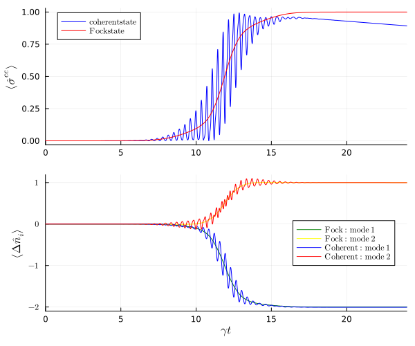

Due to the vanishing relative phase of the Fock states, the oscillations disappear.

Package versions

These results were obtained using the following versions:

using InteractiveUtils
versioninfo()

using Pkg
Pkg.status(
    [
        "QuantumInputOutput",
        "SecondQuantizedAlgebra",
        "QuantumCumulants",
        "ModelingToolkitBase",
        "OrdinaryDiffEq",
        "QuantumOptics",
        "Plots",
        "LaTeXStrings",
    ],
    mode = PKGMODE_MANIFEST,
)

Julia Version 1.12.7
Commit 6d172b025e4 (2026-08-15 08:05 UTC)
Build Info:
  Official https://julialang.org release
Platform Info:
  OS: Linux (x86_64-linux-gnu)
  CPU: 4 × AMD EPYC 7763 64-Core Processor
  WORD_SIZE: 64
  LLVM: libLLVM-18.1.7 (ORCJIT, znver3)
  GC: Built with stock GC
Threads: 4 default, 1 interactive, 4 GC (on 4 virtual cores)
Environment:
  JULIA_PKG_SERVER_REGISTRY_PREFERENCE = eager
  JULIA_DEBUG = Documenter
  JULIA_NUM_THREADS = auto
Status `~/work/QuantumInputOutput.jl/QuantumInputOutput.jl/docs/Manifest.toml`
  [b964fa9f] LaTeXStrings v1.4.1
  [7771a370] ModelingToolkitBase v1.68.2
  [1dea7af3] OrdinaryDiffEq v7.8.1
  [91a5bcdd] Plots v1.41.7
⌃ [35bcea6d] QuantumCumulants v0.7.0
  [18f9eda6] QuantumInputOutput v0.5.2 `~/work/QuantumInputOutput.jl/QuantumInputOutput.jl`
  [6e0679c1] QuantumOptics v1.2.8
⌅ [f7aa4685] SecondQuantizedAlgebra v0.10.1
Info Packages marked with ⌃ and ⌅ have new versions available. Those with ⌃ may be upgradable, but those with ⌅ are restricted by compatibility constraints from upgrading. To see why use `status --outdated -m`

This page was generated using Literate.jl.