Hong-Ou-Mandel Effect

In this example, we simulate the Hong-Ou-Mandel effect, where two single photons in identical temporal modes impinge on a 50/50 beam splitter, which leads to bunching of the photons into one output port. We perform Monte-Carlo wave function trajectories which show this behavior.

using QuantumInputOutputusing SecondQuantizedAlgebrausing QuantumOpticsusing QuantumOpticsBase: daggerusing Plotsusing LaTeXStringsusing LinearAlgebra

# symbolic Hilbert space and operatorshu1 = FockSpace(:u1)hu2 = FockSpace(:u2)hv1 = FockSpace(:v1)hv2 = FockSpace(:v2)h = hu1 ⊗ hu2 ⊗ hv1 ⊗ hv2au1 = Destroy(h, :a_u1, 1)au2 = Destroy(h, :a_u2, 2)av1 = Destroy(h, :a_v1, 3)av2 = Destroy(h, :a_v2, 4)# symbolic parameters@variables gu1::Number gu2::Number gv1::Number gv2::Number t::Real r::Real

# input cavities, beam splitter, and output cavitiesS_bs = [r t; t -r]G_u1 = SLH(1, gu1' * au1, 0)G_u2 = SLH(1, gu2' * au2, 0)G_in = G_u1 ⊞ G_u2G_bs = SLH(S_bs, [0, 0], 0)G_v1 = SLH(1, gv1' * av1, 0)G_v2 = SLH(1, gv2' * av2, 0)G_out = G_v1 ⊞ G_v2G = G_in ▷ G_bs ▷ G_out

H = hamiltonian(G)

(-0.5conj(gu1)*gv1*r)im * a_u1 * a_v1' + (-0.5conj(gu1)*gv2*t)im * a_u1 * a_v2' + (0.5conj(gv1)*gu1*r)im * a_u1' * a_v1 + (0.5conj(gv2)*gu1*t)im * a_u1' * a_v2 + (-0.5conj(gu2)*gv1*t)im * a_u2 * a_v1' + (0.5conj(gu2)*gv2*r)im * a_u2 * a_v2' + (0.5conj(gv1)*gu2*t)im * a_u2' * a_v1 + (-0.5conj(gv2)*gu2*r)im * a_u2' * a_v2

L = jump_operator(G)L[1]

conj(gu1)*r * a_u1 + conj(gu2)*t * a_u2 + conj(gv1) * a_v1

L[2]

conj(gu1)*t * a_u1 - conj(gu2)*r * a_u2 + conj(gv2) * a_v2

# Gaussian input mode (two single-photon pulses, u1 = u2)γ_ = 1.0T_p = 1 / γ_T_end = 12T_pσ = sqrt(0.5) * T_pu(t) = 1/(sqrt(σ)*π^(1/4)) * exp(-(t - 4σ)^2 / (2*σ^2))T = [0:0.002:1;] * T_endΔT = T[2] - T[1]# time-dependent couplings for input and output modesu1 = uu2 = ugu1_t = coupling_input(u1, T)gu2_t = coupling_input(u2, T)v1(t) = u(t)v2(t) = u(t)gv1_t = coupling_output(v1, T)gv2_t = coupling_output(v2, T)dict_p_t = Dict(gu1 => gu1_t, gu2 => gu2_t, gv1 => gv1_t, gv2 => gv2_t)# beam splitter parameters (50/50)η = 0.5r_ = sqrt(η)t_ = sqrt(1 - η)dict_p = Dict([t, r] .=> [t_, r_])

# numeric basisbu1 = FockBasis(1)bu2 = FockBasis(1)bv1 = FockBasis(2)bv2 = FockBasis(2)b = bu1 ⊗ bu2 ⊗ bv1 ⊗ bv2au1_qo = destroy(bu1) ⊗ one(bu2) ⊗ one(bv1) ⊗ one(bv2)au2_qo = one(bu1) ⊗ destroy(bu2) ⊗ one(bv1) ⊗ one(bv2)av1_qo = one(bu1) ⊗ one(bu2) ⊗ destroy(bv1) ⊗ one(bv2)av2_qo = one(bu1) ⊗ one(bu2) ⊗ one(bv1) ⊗ destroy(bv2)# translate to numeric operatorsH_QO = to_numeric(H, b; parameter = dict_p, time_parameter = dict_p_t)L_QO = [to_numeric(Li, b; parameter = dict_p, time_parameter = dict_p_t) for Li in L]function input_output(t, ρ)    Ht = H_QO(t)    J = [L_QO[1](t), L_QO[2](t)]    return Ht, J, dagger.(J)end

# time evolutionψ0 = fockstate(bu1, 1) ⊗ fockstate(bu2, 1) ⊗ fockstate(bv1, 0) ⊗ fockstate(bv2, 0)time, ρt = timeevolution.master_dynamic(T, ψ0, input_output)

# output observablesn_v1 = real.(expect(av1_qo' * av1_qo, ρt[end]))n_v2 = real.(expect(av2_qo' * av2_qo, ρt[end]))g2_v1 = round(real.(expect((av1_qo')^2 * (av1_qo)^2, ρt[end])) / n_v1^2, digits = 4)g2_v2 = round(real.(expect((av1_qo')^2 * (av1_qo)^2, ρt[end])) / n_v1^2, digits = 4)v1_v2_coinc =    round(real.(expect((av1_qo' * av1_qo) * (av2_qo' * av2_qo), ρt[end])), digits = 4)@show g2_v1@show g2_v2@show v1_v2_coinc

g2_v1 = 1.0
g2_v2 = 1.0
v1_v2_coinc = 0.0

We can see that the two-photon correlation for each port is one and that the correlation between the two ports is zero.

In the following, we show Monte-Carlo wave function simulations to show the bunching of photons into one of the two output ports in each realization. To this end, we collapse the photon number at the end of the time evolution ($t > 0.9 T_{end}$) with the photon detection operator in each output mode $a^{+}_{v} a_{v}$.

R = 1 # collapse raten_v1_coll(t) = (t > 0.9*T[end])*R*av1_qo'av1_qon_v2_coll(t) = (t > 0.9*T[end])*R*av2_qo'av2_qofunction input_output_mc(t, ρ)    Ht = H_QO(t)    J = [L_QO[1](t), L_QO[2](t), n_v1_coll(t), n_v2_coll(t)]    return Ht, J, dagger.(J)endNtraj = 20n_v1_mc_ls = [zeros(length(T)) for i = 1:Ntraj]n_v2_mc_ls = deepcopy(n_v1_mc_ls)

for it = 1:Ntraj    t_mc, ψt_mc = timeevolution.mcwf_dynamic(T, ψ0, input_output_mc)    n_v1_mc = real.(expect(av1_qo' * av1_qo, ψt_mc))    n_v2_mc = real.(expect(av2_qo' * av2_qo, ψt_mc))    n_v1_mc_ls[it] = n_v1_mc    n_v2_mc_ls[it] = n_v2_mcend

p1 = plot()for it = 1:Ntraj    plot!(p1, T, n_v1_mc_ls[it]; label = "")endplot!(p1; ylabel = L"\langle a^\dagger_{v_1} a_{v_1} \rangle", grid = true)p2 = plot()for it = 1:Ntraj    plot!(p2, T, n_v2_mc_ls[it]; label = "")endplot!(p2; xlabel = "time", ylabel = L"\langle a^\dagger_{v_2} a_{v_2} \rangle", grid = true)plot(p1, p2; layout = (2, 1), size = (650, 450))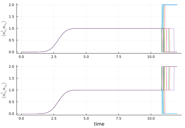

We can see that both photons always go together into one of the two detectors.

Package versions

These results were obtained using the following versions:

using InteractiveUtilsversioninfo()using PkgPkg.status(    [        "QuantumInputOutput",        "SecondQuantizedAlgebra",        "QuantumOptics",        "Plots",        "LaTeXStrings",    ],    mode = PKGMODE_MANIFEST,)

Julia Version 1.13.0
Commit d1c37793dd2 (2026-09-09 19:00 UTC)
Build Info:
  Official https://julialang.org release
Platform Info:
  OS: Linux (x86_64-linux-gnu)
  CPU: 4 × AMD EPYC 7763 64-Core Processor
  WORD_SIZE: 64
  LLVM: libLLVM-20.1.8 (ORCJIT, znver3)
  GC: Built with stock GC
Threads: 1 default, 0 interactive, 1 GC (on 4 virtual cores)
Environment:
  JULIA_PKG_SERVER_REGISTRY_PREFERENCE = eager
  JULIA_DEBUG = Documenter,Literate
  JULIA_NUM_THREADS = 1
Status `~/work/QuantumInputOutput.jl/QuantumInputOutput.jl/docs/Manifest.toml`
⌅ [7d9fca2a] Arpack v0.5.3
⌅ [861a8166] Combinatorics v1.0.2
  [d38c429a] Contour v0.6.3
⌅ [82cc6244] DataInterpolations v9.5.0
  [459566f4] DiffEqCallbacks v4.19.4
  [77a26b50] DiffEqNoiseProcess v5.36.4
  [c87230d0] FFMPEG v0.4.5
  [7a1cc6ca] FFTW v1.10.0
⌅ [53c48c17] FixedPointNumbers v0.8.6
  [069b7b12] FunctionWrappers v1.1.3
  [28b8d3ca] GR v0.73.27
  [42fd0dbc] IterativeSolvers v0.9.4
  [1019f520] JLFzf v0.1.11
  [682c06a0] JSON v1.9.0
  [0b1a1467] KrylovKit v0.10.4
  [b964fa9f] LaTeXStrings v1.4.1
  [23fbe1c1] Latexify v0.16.12
  [7a12625a] LinearMaps v3.11.4
  [442fdcdd] Measures v0.3.3
  [d8a4904e] MutableArithmetics v1.8.1
  [77ba4419] NaNMath v1.1.4
  [e7bfaba1] NumericalIntegration v0.3.4
  [1dea7af3] OrdinaryDiffEq v7.8.1
  [1344f307] OrdinaryDiffEqLowOrderRK v2.2.5
  [ccf2f8ad] PlotThemes v3.3.0
  [995b91a9] PlotUtils v1.5.0
  [91a5bcdd] Plots v1.41.7
  [aea7be01] PrecompileTools v1.3.4
  [18f9eda6] QuantumInputOutput v0.5.3 `~/work/QuantumInputOutput.jl/QuantumInputOutput.jl`
  [5717a53b] QuantumInterface v0.4.4
  [6e0679c1] QuantumOptics v1.2.10
  [4f57444f] QuantumOpticsBase v0.5.16
  [3cdcf5f2] RecipesBase v1.3.4
  [01d81517] RecipesPipeline v0.6.12
  [731186ca] RecursiveArrayTools v4.5.3
  [189a3867] Reexport v1.2.2
  [05181044] RelocatableFolders v1.0.1
  [ae029012] Requires v1.3.1
  [0bca4576] SciMLBase v3.56.1
  [431bcebd] SciMLPublic v1.3.0
  [6c6a2e73] Scratch v1.3.0
⌅ [f7aa4685] SecondQuantizedAlgebra v0.11.0
  [992d4aef] Showoff v1.1.1
  [276daf66] SpecialFunctions v2.9.0
  [90137ffa] StaticArrays v1.9.22
  [10745b16] Statistics v1.11.5
  [2913bbd2] StatsBase v0.34.13
  [789caeaf] StochasticDiffEq v7.2.0
  [d1185830] SymbolicUtils v4.48.0
  [0c5d862f] Symbolics v7.41.1
  [8ea1fca8] TermInterface v2.0.0
  [1cfade01] UnicodeFun v0.4.1
  [41fe7b60] Unzip v0.2.0
  [2a0f44e3] Base64 v1.11.0
  [ade2ca70] Dates v1.11.0
  [f43a241f] Downloads v1.7.0
  [37e2e46d] LinearAlgebra v1.13.0
  [44cfe95a] Pkg v1.13.0
  [de0858da] Printf v1.11.0
  [3fa0cd96] REPL v1.11.0
  [9a3f8284] Random v1.11.0
  [2f01184e] SparseArrays v1.13.0
  [fa267f1f] TOML v1.0.3
  [cf7118a7] UUIDs v1.11.0
Info Packages marked with ⌅ have new versions available but compatibility constraints restrict them from upgrading. To see why use `status --outdated -m`

This page was generated using Literate.jl.