Interaction Picture Scattering with a Quantum Pulse
In this example, we study the scattering of a Fock state $| n = 20 \rangle$ on a two-level system, using the interaction picture introduced in Christiansen et al., Phys. Rev. A 107, 013706 (2023). We start by loading the packages and specifying the model.
using QuantumInputOutputusing QuantumOpticsusing QuantumOpticsBase: daggerusing SecondQuantizedAlgebrausing Symbolics: Symbolicsusing SymbolicUtilsusing Plotsusing LaTeXStrings# symbolic Hilbert spacehu = FockSpace(:u)hs = NLevelSpace(:s, 2)hv = FockSpace(:v)h = hu ⊗ hs ⊗ hv# symbolic operatorsau_sym = Destroy(h, :a_u, 1)av_sym = Destroy(h, :a_v, 3)σ12_sym = Transition(h, :σ, 1, 2, 2)# symbolic parameters@variables gu::Number γ::Real gv::Number# cascade the SLH elementsG_u = SLH(1, gu' * au_sym, 0)G_s = SLH(1, sqrt(γ) * σ12_sym, 0)G_v = SLH(1, gv' * av_sym, 0)G_cas = ▷(G_u, G_s, G_v)H = hamiltonian(G_cas)(-0.5conj(gu)*sqrt(γ))im * a_u * σ₂₁ + (-0.5conj(gu)*gv)im * a_u * a_v' + (0.5gu*sqrt(γ))im * a_u' * σ₁₂ + (0.5conj(gv)*gu)im * a_u' * a_v + (-0.5gv*sqrt(γ))im * σ₁₂ * a_v' + (0.5conj(gv)*sqrt(γ))im * σ₂₁ * a_vL = jump_operator(G_cas)[1]conj(gu) * a_u + sqrt(γ) * σ₁₂ + conj(gv) * a_vUsually we deal with the above derived Hamiltonian and Lindblad. In this example, however, we transform the system into the interaction picture of the virtual cavity-cavity interaction Hamiltonian $H_{uv}$.
H_uv = hamiltonian(▷(G_u, G_v))(-0.5conj(gu)*gv)im * a_u * a_v' + (0.5conj(gv)*gu)im * a_u' * a_vTo do so, we first subtract $H_{uv}$ from $H$ and then replace the virtual cavity operators $a_v$ and $a_u$ as described in the Theory section.
H_int_sym_ = simplify(H - H_uv)# symbolic coefficient matrix $M(t)$M(i, j) = Symbolics.variable(Symbol("M_{$(i)$(j)}"); T = Complex{Real})a0_ls = [au_sym, av_sym]la = length(a0_ls)a_int_ls = [sum(M(i, j)*a0_ls[j] for j = 1:la) for i = 1:la]# substitute interaction picture operatorsint_dict = Dict([a0_ls; adjoint.(a0_ls)] .=> [a_int_ls; adjoint.(a_int_ls)])H_int_sym = simplify(substitute(H_int_sym_, int_dict))((0.5conj(gu)*imag(var"M_{11}")*sqrt(γ) - 0.5conj(gv)*imag(var"M_{21}")*sqrt(γ)) + (-0.5conj(gu)*real(var"M_{11}")*sqrt(γ) + 0.5conj(gv)*real(var"M_{21}")*sqrt(γ))im) * a_u * σ₂₁ + ((0.5gu*imag(var"M_{11}")*sqrt(γ) - 0.5gv*imag(var"M_{21}")*sqrt(γ)) + (0.5gu*real(var"M_{11}")*sqrt(γ) - 0.5gv*real(var"M_{21}")*sqrt(γ))im) * a_u' * σ₁₂ + ((0.5gu*imag(var"M_{12}")*sqrt(γ) - 0.5gv*imag(var"M_{22}")*sqrt(γ)) + (0.5gu*real(var"M_{12}")*sqrt(γ) - 0.5gv*real(var"M_{22}")*sqrt(γ))im) * σ₁₂ * a_v' + ((-0.5conj(gv)*imag(var"M_{22}")*sqrt(γ) + 0.5conj(gu)*imag(var"M_{12}")*sqrt(γ)) + (-0.5conj(gu)*real(var"M_{12}")*sqrt(γ) + 0.5conj(gv)*real(var"M_{22}")*sqrt(γ))im) * σ₂₁ * a_vL_int_sym = simplify(substitute(L, int_dict))((conj(gu)*real(var"M_{11}") + conj(gv)*real(var"M_{21}")) + (conj(gu)*imag(var"M_{11}") + conj(gv)*imag(var"M_{21}"))im) * a_u + sqrt(γ) * σ₁₂ + ((conj(gu)*real(var"M_{12}") + conj(gv)*real(var"M_{22}")) + (conj(gu)*imag(var"M_{12}") + conj(gv)*imag(var"M_{22}"))im) * a_vThe above Hamiltonian and Lindblad operator are the ones in the interaction picture of the virtual cavity interaction. We define the numerical parameters of the system, calculate the solution for the coefficient matrix $M(t)$ and solve the time evolution of the system.
# numerical parametersγ_ = 1.0n_photons = 20τ = 1 / γ_t_p = 4 / γ_u(t) = 1 / (sqrt(τ) * π^(1/4)) * exp(-0.5 * ((t - t_p) / τ)^2)T_end = 12.0T = [0:0.005:1;] * T_end# virtual-cavity couplings for input/output modesgu_t = coupling_input(u, T)gv_t = coupling_output(u, T) # identical output mode v(t) = u(t)# interaction-picture coefficient matrix M(t) for u ↔ vA_uv = coupling_matrix((gu_t, gv_t))M_t = solve_mode_evolution(A_uv, T)# constant and time-dependent parametersdict_p = Dict(γ => γ_)M_ls = [M(i, j) for i = 1:la for j = 1:la]M_t_ls = [t -> M_t(t)[i, j] for i = 1:la for j = 1:la]p_t_sym = [gu, gv, M_ls...]p_t_num = [gu_t, gv_t, M_t_ls...]dict_p_t = Dict(p_t_sym .=> p_t_num)# numerical basisbu = FockBasis(n_photons, n_photons-5)ba = NLevelBasis(2)bv = FockBasis(5)b = bu ⊗ ba ⊗ bvH_int_QO = to_numeric(H_int_sym, b; parameter = dict_p, time_parameter = dict_p_t)L_QO = to_numeric(L_int_sym, b; parameter = dict_p, time_parameter = dict_p_t)function input_output(t, ρ) Ht = H_int_QO(t) J = [L_QO(t)] return Ht, J, dagger.(J)end# time evolutionψ0 = fockstate(bu, n_photons) ⊗ nlevelstate(ba, 1) ⊗ fockstate(bv, 0)t, ρt = timeevolution.master_dynamic(T, ψ0, input_output)# numerical operatorsau = destroy(bu) ⊗ one(ba) ⊗ one(bv)av = one(bu) ⊗ one(ba) ⊗ destroy(bv)σee = one(bu) ⊗ transition(ba, 2, 2) ⊗ one(bv)n_u = real.(expect(au' * au, ρt))n_v = real.(expect(av' * av, ρt))P_e = real.(expect(σee, ρt))We can see that the mean photon number of the initial temporal mode $u$ is reduced by less than two photons. This allows us to significantly reduce the numerical Hilbert space dimension. If the interaction picture is not used, the input cavity $u$ completely empties and the output cavity almost completely fills again.
p1 = plot(T, n_u; label = L"\langle n_u \rangle")plot!( p1; xlabel = "tγ", ylabel = "excitations", ylims = (17.8, 20.2), grid = true, legend = :best,)p2 = plot(T, P_e; label = L"\langle \sigma_{ee} \rangle")plot!(p2, T, n_v; label = L"\langle n_v \rangle", ls = :dash)plot!( p2; xlabel = "tγ", ylabel = "excitations", ylims = (0, 1), grid = true, legend = :best,)plot(p1, p2; layout = (2, 1), size = (560, 420))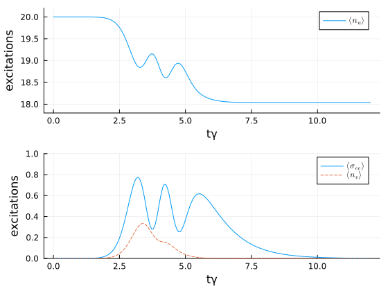
Package versions
These results were obtained using the following versions:
using InteractiveUtilsversioninfo()using PkgPkg.status([ "QuantumInputOutput", "QuantumOptics", "SecondQuantizedAlgebra", "SymbolicUtils", "Plots", "LaTeXStrings",])Julia Version 1.13.2
Commit 45b6d15e34b (2026-10-14 20:33 UTC)
Build Info:
Official https://julialang.org release
Platform Info:
OS: Linux (x86_64-linux-gnu)
CPU: 4 × Intel(R) Xeon(R) Platinum 8370C CPU @ 2.80GHz
WORD_SIZE: 64
LLVM: libLLVM-20.1.8 (ORCJIT, icelake-server)
GC: Built with stock GC
Threads: 1 default, 0 interactive, 1 GC (on 4 virtual cores)
Environment:
JULIA_PKG_SERVER_REGISTRY_PREFERENCE = eager
JULIA_DEBUG = Documenter,Literate
JULIA_NUM_THREADS = 1
Status `~/work/QuantumInputOutput.jl/QuantumInputOutput.jl/docs/Project.toml`
[b964fa9f] LaTeXStrings v1.4.1
[91a5bcdd] Plots v1.41.7
[18f9eda6] QuantumInputOutput v0.5.3 `~/work/QuantumInputOutput.jl/QuantumInputOutput.jl`
[6e0679c1] QuantumOptics v1.2.10
⌅ [f7aa4685] SecondQuantizedAlgebra v0.11.0
[d1185830] SymbolicUtils v4.53.0
Info Packages marked with ⌅ have new versions available but compatibility constraints restrict them from upgrading. To see why use `status --outdated`
This page was generated using Literate.jl.